A Matrix Based Approach for Calculating Portfolio Weights
In a previous post, I showed how to calculate and plot the efficient frontier for a set of risky assets. In this post, I extend the previous example and show how to use Octave or Matlab to calculate the portfolio weights for each of the various risky assets for any point on the efficient frontier.
In my next post, I’ll conclude this series on the efficient frontier by adding a risk free asset, showing the calculation for the tangency portfolio, and demonstrating how this creates a new frontier.
Calculating the Weights for Key Points on the Efficient Frontier
We can calculate the weights for any point on the efficient frontier once we know the weights for any two points on the efficient frontier.
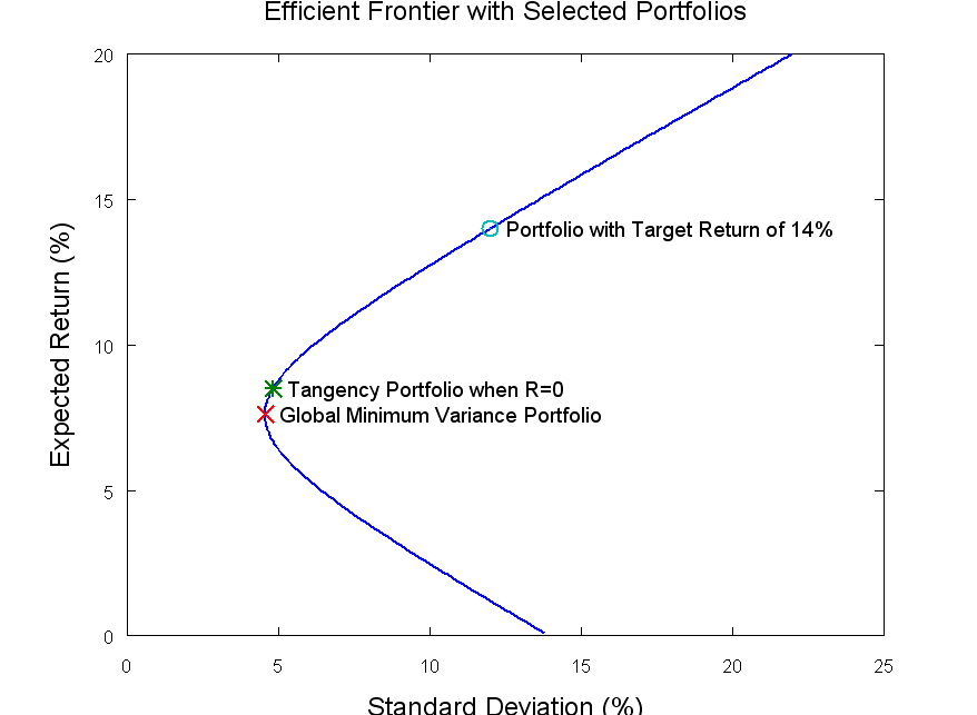
Two easy points to calculate are the global minimum variance portfolio and the tangency portfolio for the case where the risk free rate is assumed to be zero.
Global Minimum Variance Portfolio
A point of particular interest on the efficient frontier is the “global minimum variance portfolio”. This portfolio is the point on the efficient frontier which has the minimum variance or standard deviation.
We can solve for the mean and variance of the global minimum variance portfolio by setting the derivative of the equation for the variance to zero and solving for ![]() . The equations for calculating the A,B,C and
. The equations for calculating the A,B,C and ![]() values are given in the previous post.
values are given in the previous post.
![]()
Setting the derivative with respect to ![]() to zero gives:
to zero gives:
![]()
Running through all the algebra gives:
![]()
![]()
Finally, the portfolio weights for the global minimum variance portfolio are given by:
![]()
Calculating a Second Point on Efficient Frontier (Tangency Portfolio with R=0%)
We need two points on the efficient frontier to calculate any other point. We have the global minimum variance portfolio as a first point, and a second easy point to calculate is the tangency portfolio for the case where the risk-free rate is set to zero.
The equations for the expected return, standard deviations, and weights for this portfolio are given below:
![]()
![]()
![]()
The Two-Fund Separation Theorem
The two fund separation theorem states that all minimum variance portfolios on the efficient frontier are combinations of only two distinct portfolios. So, any two points on the mean variance frontier will span the set.
To calculate any point on the frontier, we can use the minimum variance portfolio and the tangency portfolio when R=0, but as a first step we need to calculate two intermediate values using the target expected return or ![]() :
:
![]()
![]()
With these values, and the portfolio weights for the two portfolios calculated above, we can find the weights for any point on the efficient frontier.
![]()
Portfolio Weights Example
As an example, we can use the four assets which I used for the example in the previous post. As a reminder, the expected returns and covariance matrix for these assets are shown below:

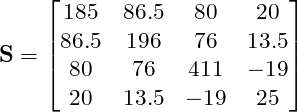
Using these assets, we can use the equations shown above to calculate the portfolio weights for the two reference portfolios, and we can then use these two portfolios to calculate portfolio weights for any point on the efficient frontier.
Global Minimum Variance Portfolio:
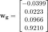
The equations presented above are implemented in an Octave script, and the portfolio weights, standard deviation, and expected return for the Global Minimum Variance Portfolio are shown below. Note that a negative portfolio weight indicates a short position in that security.
![]()
![]()
![]()
Note that this standard deviation is the minimum standard deviation for any point on the efficient frontier.
Tangency Portfolio when R=0:
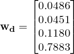
The portfolio weights, standard deviation, and expected return for the tangency portfolio when the risk free rate (R) is assumed to be zero are shown here.
![]()
![]()
![]()
Calculating Portfolio Weights for an Arbitrary Expected Return:
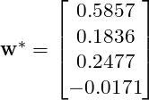
For this example, we will assume that our target portfolio return is 14%.
Using this target return, the target portfolio weights can be calculated. Again, remember that a negative portfolio weight indicates a short position in that security.
![]()
![]()
![]()
Plot of Efficient Frontier with Key Points:
Octave Code:
The script below can be run in Matlab or Octave to calculate, plot, and determine portfolio weights for any point on the efficient frontier.
By updating the expected returns (‘zbar’) and covariance matrix (‘S”), the script can be used to compute and plot the efficient frontier for any desired set of assets. It will also calculate the portfolio weights for a point on the efficient frontier with a specified target return (‘mu_tar’). The portfolio weights will be returned in the variable ‘w_s’.
clear all;
close all;

%%%%%%%%%%%%%%%%%%%%%%%%%%%%%%%%%%%%%%%%%%%%%%%%%%%%%%%%
% Mean Variance Optimizer Inputs (Update this section with your own inputs)
%%%%%%%%%%%%%%%%%%%%%%%%%%%%%%%%%%%%%%%%%%%%%%%%%%%%%%%%

% S is matrix of security covariances
S = [185 86.5 80 20; 86.5 196 76 13.5; 80 76 411 -19; 20 13.5 -19 25]

% Vector of security expected returns
zbar = [14; 12; 15; 7]

% Target Return
mu_tar = 14

%%%%%%%%%%%%%%%%%%%%%%%%%%%%%%%%%%%%%%%%%%%%%%%%%%%%%%%
% Calculating Variables
%%%%%%%%%%%%%%%%%%%%%%%%%%%%%%%%%%%%%%%%%%%%%%%%%%%%%%%

% Unity vector..must have same length as zbar
unity = ones(length(zbar),1)

% Vector of security standard deviations
stdevs = sqrt(diag(S))

A = unity'*S^-1*unity
B = unity'*S^-1*zbar
C = zbar'*S^-1*zbar
D = A*C-B^2

% Calculate Lambda and Gamma
lambda_target = (C - mu_tar*B)/D;
gamma_target =  (mu_tar*A-B)/D;

%%%%%%%%%%%%%%%%%%%%%%%%%%%%%%%%%%%%%%%%%%%%%%%%%%%%%%%
% Efficient Frontier
%%%%%%%%%%%%%%%%%%%%%%%%%%%%%%%%%%%%%%%%%%%%%%%%%%%%%%%
mu = 1:200;
mu = mu/10;

minvar = ((A*mu.^2)-2*B*mu+C)/D;
minstd = sqrt(minvar);

plot(minstd,mu,stdevs,zbar,'*')
title('Efficient Frontier with Individual Securities','fontsize',18)
ylabel('Expected Return (%)','fontsize',18)
xlabel('Standard Deviation (%)','fontsize',18)

%%%%%%%%%%%%%%%%%%%%%%%%%%%%%%%%%%%%%%%%%%%%%%%%%%%%%%%
% Global Minimum Variance Portfolio
%%%%%%%%%%%%%%%%%%%%%%%%%%%%%%%%%%%%%%%%%%%%%%%%%%%%%%%

% Mean and Variance of Global Minimum Variance Portfolio
mu_g = B/A
var_g = 1/A
std_g = sqrt(var_g)

% Minimum Variance Portfolio Weights
w_g = (S^-1*unity)/A

%%%%%%%%%%%%%%%%%%%%%%%%%%%%%%%%%%%%%%%%%%%%%%%%%%%%%%%
% Tangency Portfolio with a Risk Free Rate = 0
%%%%%%%%%%%%%%%%%%%%%%%%%%%%%%%%%%%%%%%%%%%%%%%%%%%%%%%

% Weights for Tangency Portfolio, R=0
w_d = (S^-1*zbar)/B;

% Expected Return of Tangency Portfolio
mu_d = w_d'*zbar;

% Variance and Standard Deviation of Tangency Portfolio
var_d = w_d'*S*w_d;
std_d = sqrt(var_d);

%%%%%%%%%%%%%%%%%%%%%%%%%%%%%%%%%%%%%%%%%%%%%%%%%%%%%%%
% Portfolio with Expected Return = 14%
%%%%%%%%%%%%%%%%%%%%%%%%%%%%%%%%%%%%%%%%%%%%%%%%%%%%%%%

% Weights for portfolio with target return = 14%

w_s = (lambda_target*A)*w_g + (gamma_target*B)*w_d;

% Expected Return of Target Portfolio (should match target)
mu_s = w_s'*zbar;

% Variance and Standard Deviation of target portfolio
var_s = w_s'*S*w_s;
std_s = sqrt(var_s);

%%%%%%%%%%%%%%%%%%%%%%%%%%%%%%%%%%%%%%%%%%%%%%%%%%%%%%%
% Plot Efficient Frontier and Key Points
%%%%%%%%%%%%%%%%%%%%%%%%%%%%%%%%%%%%%%%%%%%%%%%%%%%%%%%

figure
plot(minstd,mu,'linewidth',2,std_d,mu_d,'*','linewidth',2,std_g,mu_g,'x','linewidth',2,std_s,mu_s,'o','linewidth',2)
text(0.5+std_g,mu_g,'Global Minimum Variance Portfolio','fontsize',14);
text(0.5+std_d,mu_d,'Tangency Portfolio when R=0','fontsize',14);
text(0.5+std_s,mu_s,'Portfolio with Target Return of 14%','fontsize',14);
title('Efficient Frontier with Selected Portfolios','fontsize',18)
ylabel('Expected Return (%)','fontsize',18)
xlabel('Standard Deviation (%)','fontsize',18)

The methods above work for the scale/range of your percentages, but for average mu in the order of e.f. 0.0003, which are averages of log[S(t+1)/S(t)] for 5 years of data, the means are very low. Also, the standard deviations take on values of 0.01 to 0.05. Thus, the formulation appears to be range/scale dependent(?)
The program and formulas will work for any range of data. You can use the decimal values for the means and variances/covariances, and the results will be valid.
Indeed there was no scale effect observed, so you are absolutely correct.
On another note, I am using means (u_j), s.d.’s (s_j), covariance matrix based on 5 years of log[S(t+1)/S(t)] for daily price returns of 8 stocks (assets). For CAPM, I am regressing these 8 returns on the log return of the SP500 index to obtain the beta_j (j=1,1,…,8) for each. Then I set the expected excess annual return to 10%, or E(u)=0.000397 for the per/day return (0.1/sqrt(252) = 0.000397). The individual u_j’s for the stock then set to u_j = 0.000397 * beta_j
On the efficient frontier plot, the expected return (y-value) for each stock is determined as 0.000397 * beta_j, while the x-axis volatility or s.d. is simply the s_j for the stock’s 5-year log return. The efficient frontier line (efficient portfolios) is determined by incrementing E(u)=min(u_j) + i*delta, (delta= [max(u_j)-min(u_j)]/100), calculating w* for each increment using the Lagrangians, and then determining u_p and s_p via the matrix-vector and vector-matrix-vector operations on w*.
Thus far I can obtain the efficient frontier curve, and there is agreement between the greatest y-value for the curve and the stock with the greatest y=0.000397 * beta_j. However, the x-values of all of the stocks are shifted to the right and the frontier line is to the left. I have observed in the literature that for a CAPM model, the y-value plotted for each stock should be set to the fixed expected excess return you call “u” times the beta_j for each stock. Under this model, the only question becomes: how far back in the matrix algebra do you have to go for the s_j calculations when using the y=E(u)*beta_j approach to get the right values of s_j on the x-axis, that is, so the s_j’s for the frontier line directly overshadow the s_j’s for the set of stocks. There is one final point noticed on most EF plots: both the x- and y-values of the EF curve and the stock with the greatest excess return (on the far right) are always the same. So it begs, the question, when transforming u_j to u_j=E(u)*beta_j, what changes are needed to the matrix algebra above to ensure that at least both the x- and y-value for the max(y) of the EF curve and the x- and y-value for the stock with the greatest u_j are the same?
For some reason, plotting y=u*beta_j for each stock and the straightforward s_j for each stock’s 5 year log returns, the matrix algebra for w* and Lagrangians for obtaining u_p and s_p for each increment of fixed excess u
Could you steer me to the matrix equation that calculates S? It is said S=cov(x) but x is not defined. The cov(sigma)=S
Thanks
Elegant solution, one question though: How do you deal with the special case when no short selling is allowed? What will the formulas look like then? Thanks in advance.
The i,j element of the covariance matrix is the covariance of the ith and jth assets, hence the diagonal is just the variance of each asset.
Eh, I’m getting negative weights- what gives?
The solution is not restricted to positive weights. It may be that the mean variance optimal portfolio requires shorting some of the assets. These shorted assets will have negative weights.