Warning: "continue" targeting switch is equivalent to "break". Did you mean to use "continue 2"? in /home/calcul9/public_html/wp-content/themes/suffusion/functions/media.php on line 580

Warning: "continue" targeting switch is equivalent to "break". Did you mean to use "continue 2"? in /home/calcul9/public_html/wp-content/themes/suffusion/functions/media.php on line 583

Warning: "continue" targeting switch is equivalent to "break". Did you mean to use "continue 2"? in /home/calcul9/public_html/wp-content/themes/suffusion/functions/media.php on line 586

Warning: "continue" targeting switch is equivalent to "break". Did you mean to use "continue 2"? in /home/calcul9/public_html/wp-content/themes/suffusion/functions/media.php on line 589

Warning: "continue" targeting switch is equivalent to "break". Did you mean to use "continue 2"? in /home/calcul9/public_html/wp-content/themes/suffusion/functions/media.php on line 592
2012 February » The Calculating Investor
International Fama-French Portfolio and Factor Data

Regular readers know that my posts frequently utilize data from the Kenneth French data library. The data library is an excellent resource for anyone interested in the small cap and value effects and the Fama-French 3 Factor model.

Recently, I learned that the data library has been expanded to include data from developed equity markets other than the U.S. This opens up a variety of interesting possibilities for further analysis!

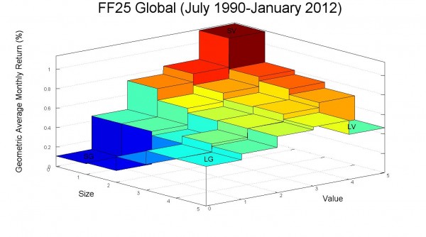
For a start, I created some plots of the small cap and value effects for each region in the new data set. The plots use the return data for the 25 portfolios sorted by size (market cap) and value (book/market).  The z-axis on each plot shows the average monthly return (geometric) for each portfolio.  The returns are U.S. dollar returns.

In a previous post, I created some similar plots for the U.S. market and provided some sample Octave code for producing these plots.

The color scale for each of the plots is tied to the magnitude of the monthly return, and the mapping between color and average return is consistent across plots. This makes it easy to compare returns between the different regions.  However, this color scaling does make the Japan plot a bit difficult to read since the average returns for Japan were much lower than the average returns for the other regions over the sample period.

The new data set also includes the Fama-French 3 Factor model factors (RMRF, HML, and SMB) for each region.  I calculated the mean, standard deviation, Sharpe ratio, standard error, and t-stat for the factors for each region and included these results in a table below each plot.

GLOBALRMRFSMBHML
Mean5.51%1.71%4.33%
Std18.91%9.33%13.65%
Sharpe0.2910.1830.317
StdE4.13%2.04%2.98%
t-stat1.330.8411.45
Continue reading »

Recommended Reading

I never completed my previously promised series on the equity risk premium, but for readers who are interested in the topic I would highly recommend the recently released “Rethinking the Equity Risk Premium” from the CFA Institute.

This free PDF contains a variety of interesting perspectives on the future of the equity risk premium. Note that a print version of the book is available on Amazon, and Kindle users can download a version formatted for Kindle for just $1.

Key Takeaway

The book has analyses from both academics and practitioners, and a variety of estimation methods are used. In my opinion, the key takeaway is that nearly all of the experts forecast future equity returns which are lower than the historical averages. Several well-argued forecasts put expected nominal equity returns in the 6%-7% per year range.

The key reason for the lower forecasts is simple. Equity valuations are higher than their average historical level. This leads to lower yields, and less potential for capital gains from further expansion of P/E ratios. Lower yields and less potential for growing valuation multiples mean that higher earnings growth must pick up the slack. Several authors provide reasons why higher-than-historical earnings growth is unlikely.  Many measurable factors actually suggest lower future economic growth (demographics, debt levels, scarce resources), and economic growth is closely linked to earnings growth. I found much of the analysis to be very convincing, though not especially uplifting!

Implications for Investors

My thoughts after reading this document are that few investors saving for retirement are prepared for equity risk premiums and real returns as low as those suggested by many of these experts. The experience of the 80s and 90s led many investors to believe that setting aside a relatively modest sum each year would lead to a comfortable nest egg by the time retirement came around. The last decade has certainly made individual investors more pessimistic about investing returns, but I’m not sure how many fully understand the impact of lower returns on their investing goals.

The table below illustrates the amount of annual savings needed to reach a one million dollar retirement goal at several different levels of nominal annual return. This simple example assumes that an investor starts saving at age 25 and continues making annual contributions through age 65 (41 contributions).  I assume that payments are made at the beginning of each year.

 
Expected ReturnTarget FV AmountRequired Annual Contribution
10%$1,000,000.00$1,863.36
8%$1,000,000.00$3,297.68
6%$1,000,000.00$5,715.90
4%$1,000,000.00$9,632.09
2%$1,000,000.00$15,658.71
Continue reading »