Warning: "continue" targeting switch is equivalent to "break". Did you mean to use "continue 2"? in /home/calcul9/public_html/wp-content/themes/suffusion/functions/media.php on line 580

Warning: "continue" targeting switch is equivalent to "break". Did you mean to use "continue 2"? in /home/calcul9/public_html/wp-content/themes/suffusion/functions/media.php on line 583

Warning: "continue" targeting switch is equivalent to "break". Did you mean to use "continue 2"? in /home/calcul9/public_html/wp-content/themes/suffusion/functions/media.php on line 586

Warning: "continue" targeting switch is equivalent to "break". Did you mean to use "continue 2"? in /home/calcul9/public_html/wp-content/themes/suffusion/functions/media.php on line 589

Warning: "continue" targeting switch is equivalent to "break". Did you mean to use "continue 2"? in /home/calcul9/public_html/wp-content/themes/suffusion/functions/media.php on line 592
Uncategorized » The Calculating Investor » Page 2
An Overview of the Equity Risk Premium

Recently, I’ve been thinking a lot about the equity risk premium, and I thought it would be an interesting topic for a series of posts.

The equity risk premium is one of the most debated topics in finance, and there are a variety of opinions about how historical return data should be interpreted and about what level of stock market returns we should expect in the future.

This first post gives an overview of the equity risk premium and discusses some possible interpretations of market valuation data. My next post (Part 2) will take a closer look at the historical data on the equity risk premium. Part 3 will look at the theory behind the equity risk premium and discuss the Equity Premium Puzzle, and Part 4 will calculate some ex-ante estimates of the equity premium using several methods.

What is the Equity Risk Premium?

The equity risk premium is defined as the difference between the overall stock market’s expected return and the risk-free rate. This risk premium compensates investors for the extra risk associated with holding stocks instead of relatively safe government bonds.

When calculating the equity risk premium, not all authors use the same measure for the “risk-free rate”.  Many authors use the t-bill rate as the risk free rate, but others argue that long-term government bonds are a better match for the duration of a company’s cash flows.

It is important to understand which measure of the risk-free rate is being used by a particular author.  Since long-term bonds rates are generally higher than t-bill rates, authors using long-term bonds as the risk-free reference will generally give lower estimates of the equity risk premium.  In this series of posts, I will use the t-bill rate as the risk-free rate. Continue reading »

What is Bitcoin?

Recently, I’ve been following the news about a new private digital currency known as Bitcoin, and I was excited to see that Planet Money had a recent podcast on this topic.

The Planet Money podcast gives an overview of Bitcoin, but this video also provides a basic introduction.

An interesting discussion on the pros and cons of Bitcoin is available on Quora.

Continue reading »
Calculating the Efficient Frontier with a Risk-Free Asset

So, I’ve been feeling a little bit bogged down on this efficient frontier topic, and I’m anxious to wrap things up with this post and move on to something more original!

In the previous two posts, I have demonstrated how to calculate the efficient frontier for any number of risky assets, and I’ve shown how to calculate the portfolio weights for each point on the efficient frontier.

In this post, I will conclude this series on the efficient frontier (finally!) by demonstrating how the frontier changes with the addition of a risk-free asset.

An example Octave script is provided for calculating and plotting the efficient frontier, capital allocation line, and tangency portfolio.

Tangency Portfolio with a Risk-Free Asset w/return R

The tangency portfolio is the intercept point if we draw a tangent line from the risk-free rate of return (on the y-axis) to the efficient frontier for risky assets. 

The equations used to calculate the portfolio weights, expected return, and variance for the tangency portfolio are shown in this section.

The variables used in these equations are described in more detail in the previous posts.  However, to review briefly, \mathbf{\bar{z}} is the vector of expected returns for the risky assets, and \mathbf{S} is the covariance matrix for the returns of these assets.  The values for A, B, C, and \Delta are intermediate values calculated using the portfolio statistics and the equations for these values are shown in my initial post on this topic.   The value R is the return on the risk-free asset.  The value \mathbf{w_{t}} is a vector showing the weight of each asset (weights sum to 1) in the tangency portfolio, and \bar{Z_{t}} and \sigma_{t}^{2} are the expected return and variance of the tangency portfolio.

\mathbf{w_{t}}=\frac{\mathbf{S^{-1}}\left ( \mathbf{\bar{z}}-R \mathbf{1}\right )}{B-AR}

\bar{Z_{t}}=\mathbf{w_{t}^{'}\bar{z}}=\frac{C-BR}{B-AR}

\sigma _{t}^{2}=\mathbf{w_{t}^{'}Sw_{t}}=\frac{C-2RB+R^{2}A}{\left ( B-AR \right )^{2}}

Continue reading »
A Matrix Based Approach for Calculating Portfolio Weights

In a previous post, I showed how to calculate and plot the efficient frontier for a set of risky assets. In this post, I extend the previous example and show how to use Octave or Matlab to calculate the portfolio weights for each of the various risky assets for any point on the efficient frontier.

In my next post, I’ll conclude this series on the efficient frontier by adding a risk free asset,  showing the calculation for the tangency portfolio, and demonstrating how this creates a new frontier.

Calculating the Weights for Key Points on the Efficient Frontier

We can calculate the weights for any point on the efficient frontier once we know the weights for any two points on the efficient frontier.

Two easy points to calculate are the global minimum variance portfolio and the tangency portfolio for the case where the risk free rate is assumed to be zero.

Global Minimum Variance Portfolio

A point of particular interest on the efficient frontier is the “global minimum variance portfolio”.  This portfolio is the point on the efficient frontier which has the minimum variance or standard deviation.

We can solve for the mean and variance of the global minimum variance portfolio by setting the derivative of the equation for the variance to zero and solving for \mu.  The equations for calculating the A,B,C and \Delta values are given in the previous post.

\sigma^2=\frac{A\mu^2-2B\mu+C}{\Delta}

Setting the derivative with respect to \mu to zero gives:

0=\frac{2A\mu-2B}{\Delta}

Running through all the algebra gives:

\mu_{g}=\frac{B}{A}

\sigma^{2}_{g}=\frac{1}{A}

Finally, the portfolio weights for the global minimum variance portfolio are given by:

\mathbf{w_{g}}=\frac{\mathbf{S^{-1}1}}{A} Continue reading »

A Matrix Based Example of  Mean-Variance Optimization using Octave

The concept of  an “efficient frontier” was developed by Harry Markowitz in the 1950s.  The efficient frontier shows us the minimum risk (i.e. standard deviation) that can be achieved at each level of expected return for a given set of risky securities.

Of course, to calculate the efficient frontier, we need to have an estimate of the expected returns and the covariance matrix for the set of risky securities which will used to build the optimal portfolio.  These parameters are difficult (impossible) to forecast, and the optimal portfolio calculation is extremely sensitive to these parameters.  For this reason, an efficient frontier based portfolio is difficult to successfully implement in practice.  However, a familiarity with the concept is still very useful and will help to develop intuition about diversification and the relationship between risk and return.

Calculating the Efficient Frontier

In this post, I’ll demonstrate how to calculate and plot the efficient frontier using the expected returns and covariance matrix for a set of securities.

In a future post, I’ll demonstrate how to calculate the security weights for various points on this efficient frontier using the two-fund separation theorem.

Calculations

In order to calculate the efficient frontier using n assets, we need two inputs.  First, we need the expected returns of each asset.  The vector of expected returns will be designated \bar{\mathbf{z}}.  The second input is the variance-covariance matrix for the n assets.  This covariance matrix will be designated as \mathbf{S}.  We also need a unity vector (\mathbf{1}) with the same length as the vector \bar{\mathbf{z}}.

Once we have this information, we can run the following calculations using a matrix based mathematical program such as Octave or Matlab.

A=\mathbf{{1}'S^{-1}1}>0

B=\mathbf{{1}'S^{-1}\bar{z}}

C=\mathbf{{\bar{z}}'S^{-1}\bar{z}}

\Delta =AC-B^{2}>0

Continue reading »

A Wealth Track Interview with Lubos Pastor

Lubos Pastor is a popular finance professor at the University of Chicago Booth School of Business.

In this interview, Professor Pastor challenges the conventional wisdom, popularized by Jeremy Siegel and others, that stock market risk decreases at longer time horizons.  He also has some interesting comments on human capital, diversification, and market efficiency.

In my opinion, Pastor’s argument about risk and horizon is a bit subtle, and it is difficult to convey in this type of an interview.  I’ve included a few links for those who want to explore this idea more thoroughly.

Original Pastor-Stambaugh Paper

Fama-French Discussion of Pastor-Stambaugh Result

Previous blog post on shortfall probability with equity premium uncertainty

Investing in America’s Most Admired Companies

Regular readers know that I believe in building a diversified investment portfolio using index funds. However, I know that there are some investors who think they can do better with a more concentrated strategy.

Many individual investors I have spoken to prefer to make concentrated bets on individual stocks, and some even have a large portion of their net worth invested in the stock of their employer!

Needless to say, I think investing a sizable percentage of your total wealth in your employer’s stock is a terrible investment strategy. Not only does it result in a poorly diversified portfolio, but in a worst case scenario you could find yourself out of a job with a worthless portfolio….remember Enron and Worldcom?

Whenever I make the case for greater diversification, the response I get it always the same: “Yes, but it’s a great company!”.   In other words, these investors acknowledge that diversification may be a good idea for other people, but they don’t believe that it applies in the case of their company.

Testing a Simple Investment Strategy

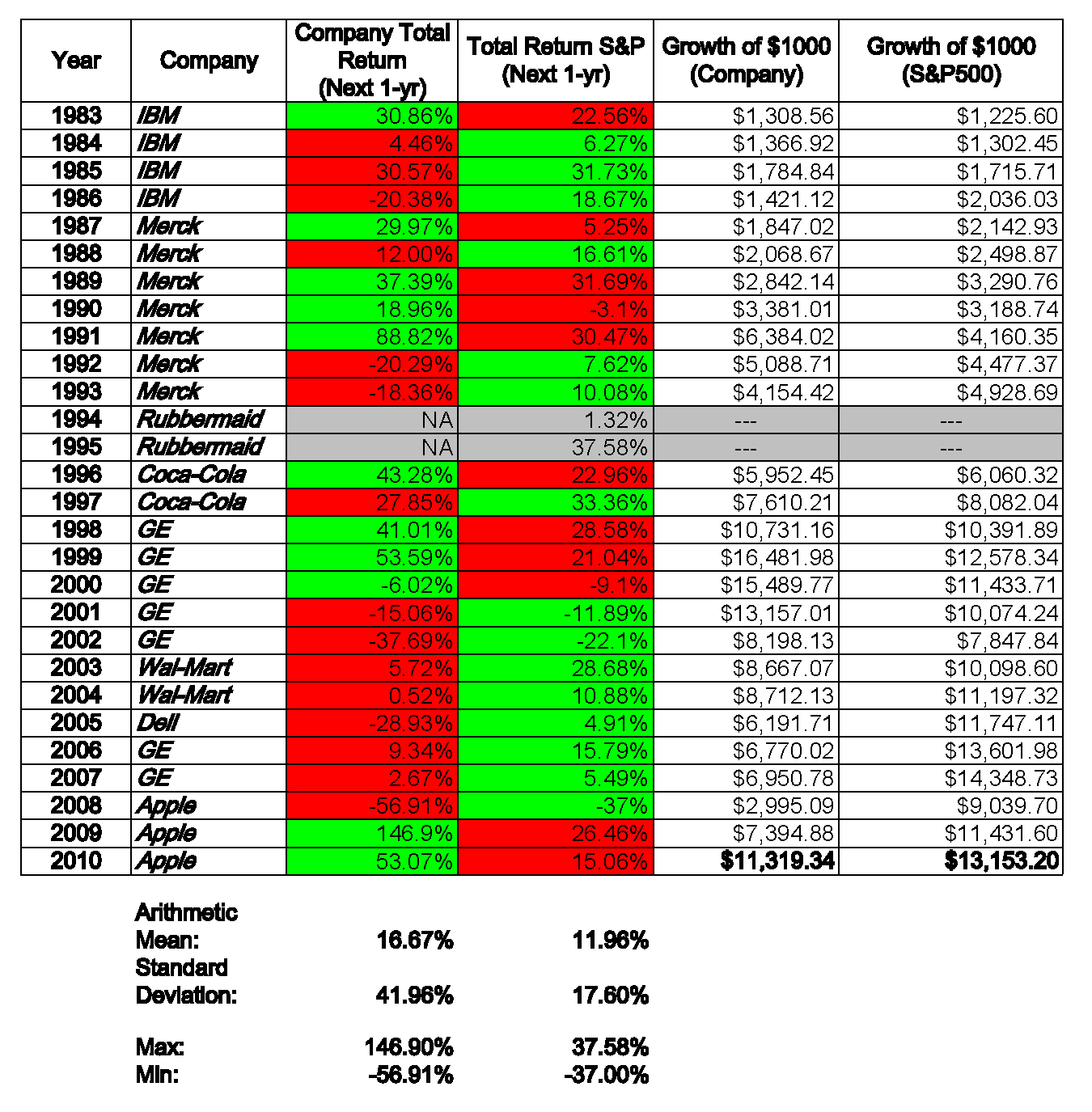
In this post, I look at the risk and return for a simple strategy that makes concentrated investments in “great companies”.   Each calendar year the strategy invests 100% of total wealth in the most admired company in America.  I’ve chosen the most admired company for each year based on a survey conducted by Fortune Magazine.

Fortune has published the list of America’s most admired companies every year since 1983.  In the table below, I’ve listed the most admired company for each year and the total return (including dividends) that the company’s stock earned in the year that it was voted to be #1.  I’ve also listed the S&P500 returns for each year.

Continue reading »

Thinking about Valuation and Mean-Reversion in the Context of a Simple Discounted Cash Flow Model

The Gordon growth model is a simple discounted cash flow (DCF) model which can be used to value a stock, mutual fund, or even the entire stock market.  The model is named after Myron Gordon who first published the model in 1959.

The Gordon model assumes that a financial security pays a periodic dividend (D) which grows at a constant rate (g). These growing dividend payments are assumed to continue forever. The future dividend payments are discounted at the required rate of return (r) to find the price (P) for the stock or fund.

Under these simple assumptions, the price of the security is given by this equation:

 P_{0}=\frac{D_{1}}{r-g}

In this equation, I’ve used the “0” subscript on the price (P) and the “1” subscript on the dividend (D) to indicate that the price is calculated at time zero and the dividend is the expected dividend at the end of period one. However, the equation is commonly written with these subscripts omitted.

Obviously, the assumptions built into this model are overly simplistic for many real-world valuation problems. Many companies pay no dividends, and, for those that do, we may expect changing payout ratios or growth rates as the business matures.

Despite these limitations, I believe spending some time experimenting with the Gordon model can help develop intuition about the relationship between valuation and return. Continue reading »

In this screencast, I demonstrate how to use R to download historical price data from Yahoo! Finance.  I also demonstrate how to convert the price data series into a return data series, and I show how to write the output to a file which can be read into a spreadsheet program such as Excel or Google Docs Spreadsheet.

I use the return data that this script generates to run CAPM and Fama-French regressions and to compute performance metrics such as Sharpe Ratios.  However, I note in the presentation that I have found that Yahoo! Finance frequently has errors in the historical price series, so users should use caution when using the return data generated from these historical prices to make financial decisions.

The code used in this screencast is pasted below, and the slides used in the screencase are available here.

# Goal: download adjusted price data for selected security, convert to returns, and write to output file

library(tseries)

# Load security data from Yahoo! Finance
prices1 <- get.hist.quote("SPY", quote="Adj", start="2005-12-25", retclass="zoo")

prices1 <- na.locf(prices1)               # Copy last traded price when NA

# To make week end prices:
nextfri.Date <- function(x) 7 * ceiling(as.numeric(x - 1)/7) + as.Date(1)
weekly.prices <- aggregate(prices, nextfri.Date,tail,1)

# To convert month end prices:
monthly.prices <- aggregate(prices1, as.yearmon, tail, 1)

# Convert weekly prices into weekly returns
r.weekly <- diff(log(weekly.prices)) # convert prices to log returns
r1.weekly <- exp(r.weekly)-1          # back to simple returns

# Convert monthly prices into monthly returns
r.monthly <- diff(log(monthly.prices))  # convert prices to log returns
r1.monthly <- exp(r.monthly)-1          # back to simple returns

# Write output data to csv file
write.zoo(r1.weekly, file="weekly.csv",sep=",",col.names=c("Dates","Percent Return"))
write.zoo(r1.monthly, file="monthly.csv",sep=",",col.names=c("Dates","Percent Return"))

I enjoy reading the discussions and debates on investment forums such as Bogleheads.org, and one very frequently discussed and debated topic is the Safe Withdrawal Rate (SWR).  

The SWR is defined as the quantity of money that can be withdrawn from a portfolio over time, including inflation adjustments, without leading to a complete depletion (i.e. failure) of the portfolio during the investor’s lifetime. 

Last week, Professor Kenneth French addressed the subject of the sustainable withdrawal rate in a video post on the Fama/French Forum website, and I’ve posted the video here:

Most SWR discussions are based on historical data or Monte Carlo simulations, which I think can be very valuable.   However, Professor French’s approach of starting with the simplest case (long-term TIPS) and building from there helps to highlight that we are taking on real risk when we stretch for higher withdrawal rates.