How confident should you be about your investment goals?
What is the probability that your investments will fall short of a particular investment goal? How is this probability affected by uncertainty about the equity risk premium?
In this post, I plan to look at a simple method for estimating the probability that a risky investment will fall short of a particular return goal, and I’ll then extend this analysis to allow for uncertainty about the equity risk premium.
This analysis is a very simplified example of the concept presented by Lubos Pastor and Robert F. Stambaugh in their paper “Are Stocks Really Less Volatile in the Long Run?”.
For starters, if we assume stock prices follow a random walk, then the probability of a risky investment underperforming a risk free investment, such as a T-bill, is given by this equation:
![]()
Where:
r = continuously compounded (log return) t-bill rate
![]() = continuously compounded (log) equity return
= continuously compounded (log) equity return
![]() = annual standard deviation of equity returns
= annual standard deviation of equity returns
T = number of years
This shortfall probability can be calculated by putting everything to the right of the greater than sign into the “normsdist” function in Excel or Google Docs.
Notice that as long as ![]() is greater than r, the probability of shortfall will approach zero for large values of T. So, for this model, the risk of falling short of an investment goal will approach zero if the horizon is long enough and the mean return is greater than the t-bill return.
is greater than r, the probability of shortfall will approach zero for large values of T. So, for this model, the risk of falling short of an investment goal will approach zero if the horizon is long enough and the mean return is greater than the t-bill return.
Now, if we add equity premium uncertainty, the shortfall probability is given by this equation:
![]()
The additional ![]() term is the standard deviation of our estimate of the equity premium. Again, the probability can be calculated using the “normsdist” function.
term is the standard deviation of our estimate of the equity premium. Again, the probability can be calculated using the “normsdist” function.
Notice that in this model, the probability will not approach zero for large values of T. There is a limit to how small the probability can become which is dependent on our uncertainty about the equity premium.
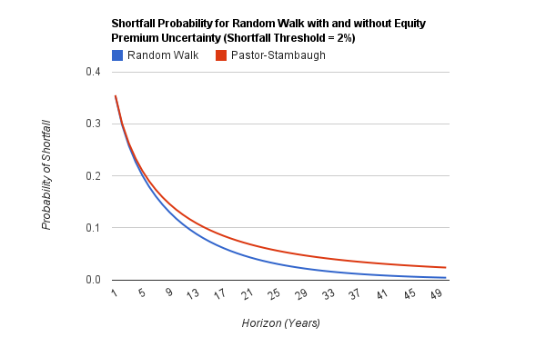
I plotted both shortfall probabilities vs. horizon for an assumed equity return of 8% and 16% standard deviation, and risk-free rate of 2%. I also used 2% as the sigma for the equity premium uncertainty.
Here is the plot for shortfall probability vs. horizon.
Clearly, the risk of a shortfall is elevated when we include the equity premium uncertainty. However, the difference does not appear to be huge. The probability of underperforming the risk free rate is still small at long horizons.
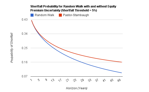
We can also substitute a minimum return goal for the risk free rate to calculate the probability of not meeting a particular return goal. For example, if I need a return of at least 5% to meet my goals for retirement, then, keeping the other parameters the same as above, the shortfall probability is shown by this plot.
In this example, the effect of the equity premium uncertainty is larger. Over a 40-50 year horizon, there is a very meaningful difference between the two methodologies.
These examples are only intended to illustrate the effect of equity premium uncertainty as compared to the pure random walk case. The examples don’t consider the potential for mean-reversion or fat tailed return distributions. Also, it is very important to note that they don’t consider the magnitude of the shortfall. For example, if your probability of falling short is 10%, the magnitude of this shortfall might be very small or it might be huge. This method of analysis ignores this consideration, but you can get a sense of the expected shortfall by experimenting with equations using a variety of return thresholds.
My spreadsheet for generating these graphs can be accessed using Google Docs. If you save a copy of this document, it can be modified to incorporate your own assumptions and the effect of equity premium uncertainty can be evaluated under a variety of scenarios.


Thanks a lot for this blog. do you have same elaboration for mean absolute minimization model and tracking error minimization model?
[…] details for the number crunching are straightforward. Several years ago The Calculating Investor outlined the procedure with an Excel spreadsheet. Let’s expand the concept a bit by applying the normal […]
[…] details for the number crunching are straightforward. Several years ago The Calculating Investor outlined the procedure with an Excel spreadsheet. Let’s expand the concept a bit by applying the normal […]