Two Common Questions
Over the past few weeks, gasoline prices have been a frequent conversation topic. The rapid rise in prices has hit most of us in the pocketbook, and it has caused wannabe economists such as myself to ponder the relationship between oil and gasoline prices.
In this post, I’m going to look at two common questions to see if we can reach any conclusions.
Question #1: What is the relationship between Oil Prices and Gasoline Prices?
This is a relatively easy question to answer. The data on oil prices is available on the EIA website, and the same website has data on retail gasoline prices for a variety of cities and regions. Since I am a Chicago resident, I chose to run the regression using the retail gasoline price series for Chicago.
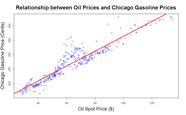
This plot shows the last seven years of oil and gasoline prices. The blue dots are the weekly price data points and the red line is the fitted regression line.
The equation for the regression line is shown here:
![]()
So, roughly speaking, the price of gasoline will go up by about a quarter for each $10 increase in the price of a barrel of oil.
The R-squared for this regression is 0.87. A close examination of the data shows some seasonality in the regression residuals, so we could probably improve this model by adding a dummy variable for the summer months when a special blend of gasoline is required in the Chicago metropolitan area. However, this simple version of the equation is a good first approximation.
Question #2: Do gasoline prices respond more quickly when oil prices go up than when they fall?
I often hear the complaint that gasoline prices go up immediately when the price of oil rises, but they do not go down immediately when the price of oil falls. I decided to check the data to see whether or not this was true.
Here is the methodology:
The relationship used in the Oil-Gas price equation developed in Question #1 (G = retail gasoline price, O=oil price per barrel) is:
![]()
So, the change in gasoline prices resulting from a change in oil prices is:
![]()
This can be further separated to distinguish the positive changes in oil price from the negative changes.
![]()
Where:
![]()
![]()
![]()
![]()
A more general version of this equation is:
![]()
In this model specification, there are two leading terms and three lagging terms. If we run this regression, the coefficients should be symmetrical for the positive and negative change series if the response of gasoline prices is symmetric for both oil price increases and oil price decreases. If there is a difference in the up and down coefficients then this would indicate that gasoline prices respond differently to positive oil price shocks than they do to negative oil price shocks.
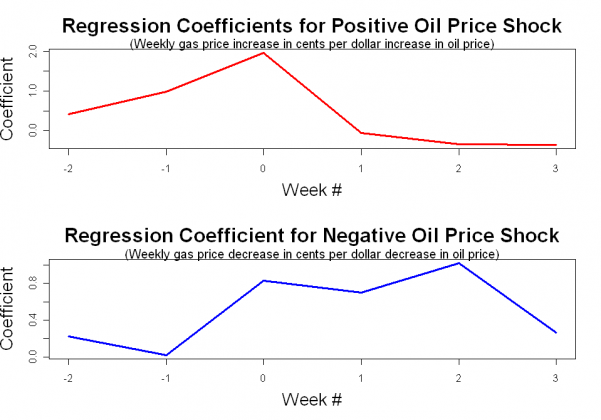
The plots of the regression coefficients is shown here:
How to interpret this plot: The red line shows the response to a positive oil price change. The magnitude represents the weekly increase in gasoline price (in cents) for a $1 increase in oil price at week 0. The blue line shows the response to a negative oil price change. The magnitude represents the weekly decrease in gasoline price (in cents) for a $1 decrease in the oil price at week 0.
Notice that most of the increase in gasoline price occurs contemporaneously with the oil price increase, while a decrease in gasoline prices is spread out over several weeks. In the case of an increase, the gasoline price increase actually seems to lead the oil price increase a bit. This is at least partly a result of the weekly measurement dates of the EIA oil price series being offset from measurement dates for the EIA retail gasoline price series. Clearly, these two responses are not symmetric!
The bottom line is that this graph shows that gasoline prices do respond more rapidly when oil prices increase than when oil prices decrease!
Additional Info:
The regression method used to test the gasoline price response was based on the method used in this paper comparing wholesale and retail gasoline prices. Also, I found that there are several academic papers demonstrating the asymmetry between oil and gas price changes, and a nice example is available here.
The full regression results are shown here:
| Name | Coefficient | Standard Error | t-value | Pr(>|t|) | Significance |
|---|---|---|---|---|---|
| (Intercept) | 0.42957 | 0.82627 | 0.52 | 0.603464 | |
| Positive Week -2 | 0.41661 | 0.26411 | 1.577 | 0.115593 | |
| Positive Week -1 | 0.97618 | 0.27402 | 3.562 | 0.000418 | *** |
| Positive Week 0 | 1.96498 | 0.27415 | 7.168 | 4.49E-12 | *** |
| Positive Week +1 | -0.06072 | 0.27796 | -0.218 | 0.827216 | |
| Positive Week +2 | -0.35566 | 0.27482 | -1.294 | 0.196451 | |
| Positive Week +3 | -0.36709 | 0.27371 | -1.341 | 0.180724 | |
| Negative Week -2 | 0.22187 | 0.25144 | 0.882 | 0.378162 | |
| Negative Week -1 | 0.01976 | 0.26145 | 0.076 | 0.939804 | |
| Negative Week 0 | 0.82732 | 0.26464 | 3.126 | 0.001918 | ** |
| Negative Week +1 | 0.70322 | 0.26375 | 2.666 | 0.008023 | ** |
| Negative Week +2 | 1.02332 | 0.26396 | 3.877 | 0.000126 | *** |
| Negative Week +3 | 0.26196 | 0.25395 | 1.032 | 0.303006 |
The R-squared of this regression was 0.4045.
The R code used in the analysis is shown here:
# Oil-Gas Price Comparison

# Load data; the csv file was constructed from data on the EIA website
x <- read.csv("oil_gas2.csv")

gas   <- x[,2]
oil   <- x[,3]
gasus <- x[,5]
dates <- x[,1]

# Chicago Oil and Chicago Gasoline Prices
out1 <- lm(gas ~ oil)
summary(out1)

windows()
plot(oil, gas,xlab="",ylab="",col="blue")
abline(out1,col="red",lwd=3)
title("Relationship between Oil Prices and Chicago Gasoline Prices",xlab="Oil Spot Price ($)",ylab="Chicago Gasoline Price (Cents)",cex.main="2.0",cex.lab="1.75")

# Difference and Lags
diffgas <- rev(diff(gas))
diffoil <- rev(diff(oil))

# Construct leading and lagging oil price series
lead2 <- c(0,0,diffoil)
lead1 <- c(0,diffoil)
lag1 <- diffoil[2:length(diffoil)]
lag2 <- diffoil[3:length(diffoil)]
lag3 <- diffoil[4:length(diffoil)]
lag4 <- diffoil[5:length(diffoil)]

lead2 <- lead2[3:length(lag4)]
lead1 <- lead1[3:length(lag4)]
lag0 <- diffoil[3:length(lag4)]
lag1 <- lag1[3:length(lag4)]
lag2 <- lag2[3:length(lag4)]
lag3 <- lag3[3:length(lag4)]
lag4 <- lag4[3:length(lag4)]

# Regression with leading and lagging terms
out2 <- lm(diffgas[3:(length(lag4)+2)] ~ lead2 + lead1 + lag0 + lag1 + lag2 + lag3 + lag4)
summary(out2)

# Separate out positive and negative terms from leading and lagging oil series
plead2 <- pmax(lead2,0)
plead1 <- pmax(lead1,0)
plag0 <- pmax(lag0,0)
plag1 <- pmax(lag1,0)
plag2 <- pmax(lag2,0)
plag3 <- pmax(lag3,0)
plag4 <- pmax(lag4,0)

nlead2 <- pmin(lead2,0)
nlead1 <- pmin(lead1,0)
nlag0 <- pmin(lag0,0)
nlag1 <- pmin(lag1,0)
nlag2 <- pmin(lag2,0)
nlag3 <- pmin(lag3,0)
nlag4 <- pmin(lag4,0)

out3 <- lm(diffgas[3:(length(lag4)+2)] ~ plead2 + plead1 + plag0 + plag1 + plag2 + plag3 + nlead2+ nlead1 + nlag0 + nlag1 + nlag2 + nlag3)
summary(out3)

windows()
par(mfrow=c(2,1))
xval=-2:3
plot(xval,out3$coefficients[2:7],lwd=3,col='red',type='l',xlab="",ylab="")
title("Regression Coefficients for Positive Oil Price Shock",xlab="Week #",ylab="Coefficient",cex.main="2.0",cex.lab="1.75")
mtext("(Weekly gas price increase in cents per dollar increase in oil price)",cex=1.25)
plot(xval,out3$coefficients[8:13],lwd=3,col='blue',type='l',xlab="",ylab="")
title("Regression Coefficient for Negative Oil Price Shock",xlab="Week #",ylab="Coefficient",cex.main="2.0",cex.lab="1.75")
mtext("(Weekly gas price decrease in cents per dollar decrease in oil price)",cex=1.25)
G3RJJPQ4MHXV


I’m a little surprised that the relationship is linear. I thought tax was usually on a per gallon bases. Also, the fixed costs of the infrastructure for refining crude oil to gasoline should not change that much as crude oil price changes.
Why not use an asymmetric price transmission model?
Also how well does your model fit the data when you back test it?