Why I am skeptical about the “rebalancing bonus” even though I believe that “buy, hold, and rebalance” is a great investment strategy
This past week, Rick Ferri, the Founder of Portfolio Solutions, wrote an interesting blog post on Forbes.com titled “Passive Investing Beats the Markets”. In the post, Mr. Ferri argues that a buy, hold, and rebalance strategy using low cost index funds outperforms a number of other strategies including an index-based strategy of buy, hold, and never rebalance.
In a related discussion on Bogleheads.org, Mr. Ferri provided some historical data supporting this conclusion, but I thought I would take a stab at running some simulations to better understand the conditions where rebalancing can boost total returns.
The Bernstein Analysis of the Rebalancing Bonus
In 1997, William Bernstein published an analysis on his website which showed how the “rebalancing bonus” was affected by the difference in average returns between two securities and the correlation between those returns.
Bernstein’s analysis showed that rebalancing can increase returns when two volatile securities have similar average returns and low correlation. The intuition behind this result is straighforward, if two securities are highly correlated, then there is little opportunity to transfer funds from the security which is performing relatively well to the security that is performing relatively poorly. If the securities have low correlation, then there are more frequent opportunities to “buy low, sell high” through rebalancing.
Similarly, if the two securities have very different average returns, then the rebalancing will, on average, move funds from the security with higher average returns to the security with lower average returns. This is obviously not a strategy which will boost total returns over time, although it may make sense for risk management purposes.
Rebalancing Simulations
The plots below are based on Monte Carlo simulations of two securities whose returns follow a random walk. These simulations are similar to the Monte Carlo simulations that Bernstein used in his original 1997 analysis, but I’ve added a correlation factor to the simulations.
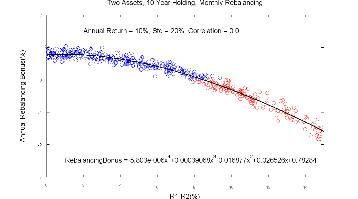
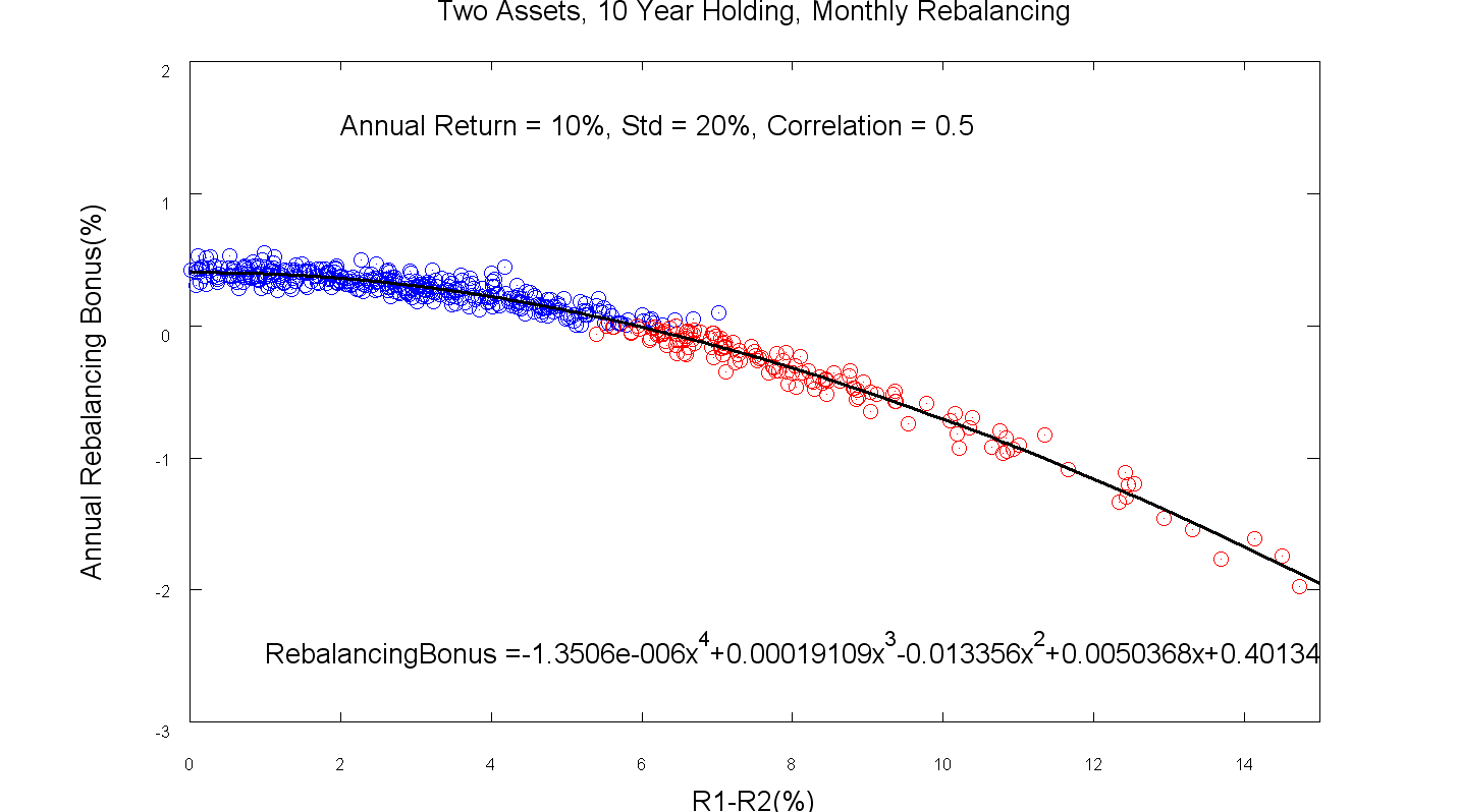
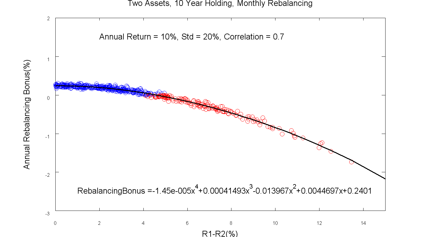
The x-axis in these plots shows the difference in the average returns of the two securities in each run of the simulation. The y-axis of the plot shows the rebalancing “bonus” or “penalty”. In other words, the y-axis shows the average annual difference in returns between a portfolio split evenly between the two securities and rebalanced monthly, and a portfolio split evenly between the two securities which is never rebalanced.
I’ve shown the instances where the simulation produced a rebalancing bonus in blue, and I’ve shown the simulation runs where there was a rebalancing penalty in red. The black line is a polynomial which is fitted to the simulation results. The equation for the fitted line is included in each plot.
In the first plot, the returns of the two securities have a correlation of zero. The simulation uses a target return of 10% for each security, and the standard deviation for each security is 20% per year. These parameters are similar to long term average return and standard deviation for the S&P500 and other developed country indexes.
With a correlation of zero, the rebalancing bonus almost 1% per year, and there is a positive rebalancing bonus even if the return difference between the two securities is as large as 8% per year.
However, finding two high-return asset classes with a correlation of zero is no easy task. If the correlation is increased to 0.5, the rebalancing bonus is reduced to 0.5% annually, and the return difference over ten years must be less than 6% annually.
Increasing the correlation to 0.7, reduces the maximum annual rebalancing bonus to about 0.2%, and the bonus stays positive up to a return difference of 4% per year. At this level of correlation, the rebalancing bonus could easily be wiped out if the investor incurred fees and taxes as part of the rebalancing process.
Rising Correlations: Looking at the Trends
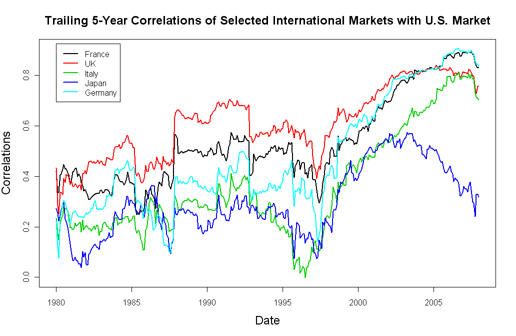
As shown in the previous section, the rebalancing bonus depends on a low correlation between the securities in the portfolio.
Let’s take a look at the trend in correlations for global markets. The international stock return data is taken from the Kenneth French website. This data starts in 1975, and I’ve chosen the 5 countries with the highest GDP (other than the U.S.) in 1975. The trailing 5-year correlation of each country’s monthly market returns with the U.S. market monthly returns is shown in the plot below. Clearly, with the exception of Japan, the correlations have been rising over time.
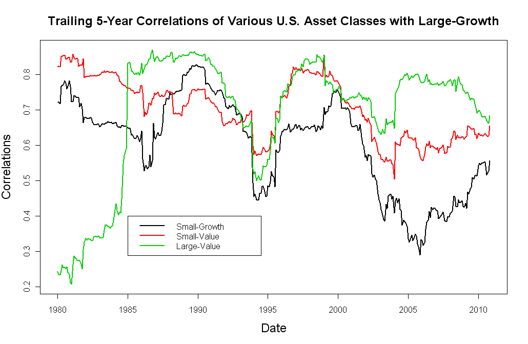
I have also looked at the correlations within the U.S. market. I ran correlations between the most extreme portfolios in the Fama-French 25 portfolios. These portfolios were sorted by value and size characteristics, so this plot shows the correlation between Large-Growth (similar to S&P500) and the Large-Value, Small-Growth, and Small-Value portfolios.
These correlations do not show the rising trend that we saw with the international markets, but the correlations are high enough to cut into the potential for a rebalancing bonus. Also, these plots show correlations for the most extreme portfolios in the Fama-French 25 portfolios. In practice, most small cap and value funds are not as extreme as these portfolios, and they would show even higher correlation with the overall market.
Conclusion
My purpose in this post has not been to show that a rebalancing bonus is impossible or even that it is extremely unlikely. However, I do believe that although rebalancing has historically improved both risk-adjusted and total returns, investors should be aware that a meaningful rebalancing bonus may be harder to come by in a future of more integrated (and correlated) capital markets. This will be especially true if trading costs and taxes are incurred as part of the rebalancing process.
Despite this conclusion, I continue to believe buy, hold, and rebalance will continue to be an excellent strategy for managing the risk of a diversified portfolio.
Additional Information:
The Octave code used for the Monte Carlo simulations is shown here:
clear all;
close all;

n=120;
s1 = 0.05; % Monthly Standard Deviation
s2 = 0.05; % Monthly Standard Deviation
m1 = 0.00833; % Monthly Return
m2 = 0.00853; % Monthly Return
p = 0.0; % Correlation between assets
exceedcount = 0;
undercount = 0;

u = randn(1,n);
v = randn(1,n);
x = s1*u+m1;
y = s2*(p*u+sqrt(1-p^2)*v)+m2;

for i = 1:500
    u = randn(1,n);
    v = randn(1,n);
    x = s1*u+m1;
    y = s2*(p*u+sqrt(1-p^2)*v)+m2;
    z = 0.5*(x+y);
    norebalance(i) = 0.5*(prod(1+x)-1) + 0.5*(prod(1+y)-1);
    rebalance(i) = prod(z+1) - 1;
    bonus(i) = ((rebalance(i)+1)^(1/10)-1) - ((norebalance(i)+1)^(1/10)-1);
    rdiff(i) = abs((prod(1+x)^(1/10)-1) - (prod(1+y)^(1/10)-1));
    if (bonus(i) > 0)
        exceedcount = exceedcount +1;
        pos_bonus(exceedcount) = bonus(i);
        pos_diff(exceedcount) = rdiff(i);
    end
    if (bonus(i) <= 0)
        undercount = undercount + 1;
        neg_bonus(undercount) = bonus(i);
        neg_diff(undercount) = rdiff(i);
    end
end

% Fitted Curve
coeffs = polyfit(100*rdiff,100*bonus,4)
yvals = polyval(coeffs,100*rdiff)

plot(100*pos_diff,100*pos_bonus,'o3',100*neg_diff,100*neg_bonus,'o1')
pause(5)
axis([0 15 -3 2])
title('Two Assets, 10 Year Holding, Monthly Rebalancing','fontsize',20);
ylabel('Annual Rebalancing Bonus(%)','fontsize',20)
xlabel('R1-R2(%)','fontsize',20)

% Add Fitted Polynomial to Plot
sortx = sort(rdiff)
sorty = fliplr(sort(yvals))
line(100*sortx,sorty,'linewidth',3)

equation = strcat('RebalancingBonus = ',num2str(coeffs(1)),'x^4+',num2str(coeffs(2)),'x^3',num2str(coeffs(3)),'x^2+',num2str(coeffs(4)),'x+',num2str(coeffs(5)))
text(1,-2.5,equation,'fontsize',20)
text(2,1.5,'Annual Return = 10%, Std = 20%, Correlation = 0.0','fontsize',20)

I agree that rebalancing is not the layup that many people see it as. Investors like to think in terms of reversion to the mean which gets you to automatically sell the pricier asset and buy the cheaper asset. When that is brought up I mention the case of Japan. The cheaper asset can continue to get cheaper for a long time.
The point about transactions costs is important. The bottom line is to me is that rebalancing can add value but it is not a no-brainer. There is still a bit of analysis that needs to be done.
Yes, Japan is a great example, and I like the “not a lay-up” metaphor. Rebalancing has often increased returns in the past, and I hope it increases returns in the future as well…but I do think that investors should be aware that the necessary conditions for increased returns are a bit fragile.
Jack Bogle has some interesting comments along these lines on his website in his response to “Mr. M”: http://johncbogle.com/wordpress/2007/06/15/john-bogle-responds-to-ask-jack-questions-2/