Tutorial: The Capital Asset Pricing Model

Let’s begin with some Q&A:

Question: Why do some financial assets tend to earn higher returns than others?

Answer: Financial theory tells us that, on average, higher returns are earned by financial assets that have higher risk.

Question: Ok, so how do we measure risk?

Answer: One model used for measuring risk is the Capital Asset Pricing Model or CAPM.   In the CAPM, the risk that a security contributes to a diversified portfolio is measured by its beta (or ), and the expected excess return of the security is proportional to beta.

The term “excess return” refers to the additional return that the security earns above the risk-free rate.  For U.S. investors, the t-bill rate is typically used as the risk-free rate.

The excess return earned by the market portfolio is also known as the “market risk premium”.  The risk premium for an individual security may be higher or lower than the market risk premium depending on the security’s beta.

If the beta is greater than one (the beta of the market portfolio is one by definition), then the expected return for the security is higher than the market average, and, if the beta is less than one, the expected return is lower.

In the CAPM, the total expected return of a security is given by this equation:

Notice that only the excess return varies with beta, and the risk free rate is added to the security’s risk premium to get the total expected return.

The variables in this equation are:

The “expected return” is the return that the investors expect to earn on average given the current price of the security.  Of course, the expected return is what should happen on average over the very long term, but in any given period the realized return may be very different than the expected return.

All else equal, the expected return is related to price.  If the price rises, and our expectations of the future cash flows from the security are unchanged, then our expected return falls since we are paying more for the same future future cash flows.  Similarly, if the price falls, and our expectations for future cash flows are unchanged, then the expected return will rise.

Question:  What the heck is Beta?

Answer: Beta is a statistical measure which captures the relationship between the returns of a security and the returns of the overall market.  Beta is calculated as the covariance between the security’s excess returns and the excess returns of the market portfolio divided by the market portfolio variance.

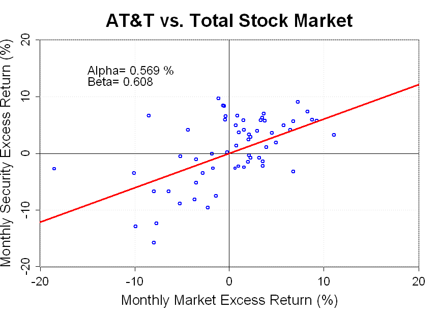
Confused?  This can be more simply illustrated in the graph below.  I’ve created a scatter plot showing the last 5-years of monthly excess returns on AT&T  stock and the monthly excess market returns.

The red line is the best fit line showing the relationship between the market’s excess returns and AT&T’s excess returns. The slope of this line is the beta of AT&T. In this case, the beta is equal to 0.608, which means that when the market rises or falls by 1% the stock of AT&T tends to rise or fall by about 0.608%.

Obviously, the regression relationship between the AT&T return and the market return  is far from perfect.  Many of the scatter plot points showing the actual returns for AT&T and the market portfolio fall far from the best fit line.  However, according to the CAPM these “errors” should average out in a diversified portfolio.

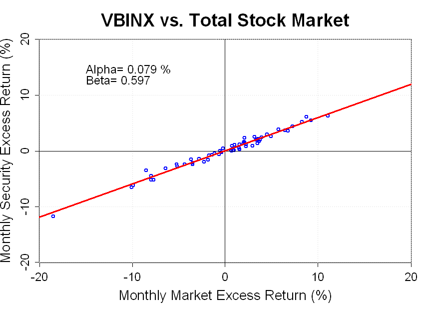
As an example, lets look at the Vanguard Balanced Index Fund.  This fund contains a diverse portfolio of both stocks and bonds, and the beta of the fund is very similar to the beta of AT&T stock.

Notice that all the scatter plot points in the second graph fall very close to the regression line.  We don’t see the large errors that were seen in first graph.  The “diversifiable” risk has been eliminated and we are left only with a “non-diversifiable” exposure to overall market risk which is defined by the average beta of the securities in the portfolio.

Question:  Why should we expect average returns to be proportional to beta?

Answer: Start by assuming that we lived in a world where the average return of a stock was not proportional to its beta.  In this case, a smart investment strategy might involve buying a diversified portfolio of low beta stocks.  As with VBINX, the diversifiable risk would be eliminated by combining many stocks, and we would end up with a portfolio which had low sensitivity to the ups and downs of the overall market (i.e. low beta), but had a similar average return to the market.

Does this scenario seem too good to be true?  If it were possible to construct a low-beta portfolio with average returns equal to the market return, then this would be very desirable portfolio for any risk averse investor.  Investors would buy this low risk portfolio (driving up the price of low beta stocks) and they would avoid the high beta stocks which could increase the market risk of the portfolio (driving down the price of high beta stocks).

This arbitrage process would drive down the returns of low beta stocks and drive up the returns of high beta stocks until an equilibrium was reached.  In fact, the CAPM makes the argument that constant trading and instant incorporation of new information keeps markets in exactly this type of an equilibrium, and it follows that low-beta stocks should, on average, earn lower returns than high-beta stocks.

Question:  Ok, so what is alpha?

Answer: In the CAPM, alpha is a risk-adjusted measure of return.  It measures the extent to which a security’s return exceeds or falls short of the return predicted by the CAPM.  A positive alpha indicates that, after adjusting for exposure to market risk, a security has outperformed the market portfolio.

Alpha can be measured using the following regression:

The R-script I have included below, can be used to run this regression on a stock or fund.

If the CAPM is a good model, we would expect that broadly diversifed portfolios should have alphas that are close to zero.  If we are able to sort stocks into portfolios which consistently generate a significantly positive or negative alpha then this would indicate a problem with the model.

Question: So, does the CAPM actually work?

Answer: The CAPM aims to describe the average relationship between risk and return.  It does not disprove the CAPM if individual stocks have returns which are well above or below what is predicted by their betas since there is a lot of diversifiable risk in any individual security.

However, if we can find broadly diversified portfolios which consistently generate returns above or below what is predicted by the CAPM, then we have grounds to question the model.

In practice, several “anomalies” to the CAPM such as the “size” and “value” effect are well documented, and more sophisticated models such as the Fama-French Three Factor model have been developed to account for these anomalies.

Conclusion:

The CAPM is a useful and important model.  It gives us a formal relationship between risk and return, and it creates a distinction between diversifiable and non-diversifiable risk.  These concepts are crucial to a solid understanding of modern finance.

Nevertheless, the CAPM is far from perfect.  Research has shown that market risk is not the only risk that investors care about, and more sophisticated asset pricing models have been developed.  However, all of these models build on the important concepts developed in the CAPM.

Additional Info:

Data: The data for AT&T returns and VBINX returns was taken from Yahoo! Finance, and the market return and risk-free rate was taken from the Kenneth French website.

Code: The R-code used to generate the plots is shown below.

# Goal: Estimate CAPM alpha and beta for individual stocks and create regression plot
# using monthly returns

library(tseries)

# Load FF factor returns
startyear <- 2006
startmonth <- 1
endyear <- 2010
endmonth <- 12

start <- (startyear-1926.5)*12+startmonth
stop <- (endyear - 1926.5)*12+endmonth

ff_returns <- read.table("F-F_Factors_monthly.txt")
rmrf <- ff_returns[start:stop,2]/100
rf <- ff_returns[start:stop,5]/100

# Load security data from Yahoo! Finance
prices1 <- get.hist.quote("VBINX", quote="Adj", start="2005-12-25", retclass="zoo")

prices1 <- na.locf(prices1)               # Copy last traded price when NA

# To make monthly returns, you must have this incantation:
monthly.prices <- aggregate(prices1, as.yearmon, tail, 1)

# Convert selected monthly prices into monthly returns to run regression
r <- diff(log(monthly.prices))  # convert prices to log returns
r1 <- exp(r)-1                  # back to simple returns

# Now shift out of zoo into ordinary matrix
rj <- coredata(r1)
rj <- rj[1:60]  # cutoff data at 60 months, I'm using data from Jan 2006-Dec 2010
rjrf <- rj - rf

d <- lm(rjrf ~ rmrf)               # CAPM model estimation.
print(summary(d))                  # Print regression results

# Scale up returns so they can be plotted as percents
rM <- 100 * rmrf
rj <- 100*rjrf

# Make a plot
dev.new(width=9,height=6.5)
big <- max(abs(c(rj, rM)))
range <- c(-big, big)
plot(rM, rj, xlim=range, ylim=range,xlab="", ylab="",col="blue",lwd=2,cex.axis=1.5)
title("VBINX vs. Total Stock Market",xlab="Monthly Market Excess Return (%)",ylab="Monthly Security Excess Return (%)",cex.main="2.25",cex.lab="1.75")
grid()
abline(h=0, v=0)
# Add regression line
abline(coefficients(d),lwd=3,col="red")

# Include Alpha and Beta estimate in plot
a <- round(d$coef[1]*100,3)
b <- round(d$coef[2],3)
alpha <- paste("Alpha=",a,"%")
beta <- paste("Beta=",b)
text(-15,14,alpha,adj=c(0,0),cex=1.5)
text(-15,12,beta,adj=c(0,0),cex=1.5)