PCA Factors vs. Fama-French Factors

In my previous post, I showed how to create equity return factors using principal component analysis. In this post, I’m going to compare the three PCA factors I created to the three Fama-French factors.

The goal of this post is to determine whether or not the Fama-French factors are leaving anything significant on the table that the PCA factors, which capture as much covariance in the target portfolios as is possible with three factors, are able to pick up.

In other words, I’ll be comparing the R^2s and alphas for both the Fama-French factors and the PCA factors, and, after some re-arranging, I’ll also compare the factor loadings.

Data

The Fama-French 3 Factor (FF3F) data and the Fama-French 25 size and value sorted portfolio (FF25) data come from the Kenneth French website.  The PCA factors were calculated in the previous post, and I posted the data in a Google Docs Spreadsheet.

R^2 and Alpha using PCA Factors and Fama French Factors

As a first step, the R^2s and alphas for the FF25 portfolios can be calculated using both the Fama-French factors and the PCA factors.

The PCA factors will give us the best fit across the 25 portfolios that is possible with three factors, so we expect the R^2s for the Fama-French factors to be lower on average. The question is: How much lower?

The tables below show the R^2s for the PCA Factors and Fama-French Factors.  For each table, the values highlighted in green have an R^2 which is higher than the alternative model, and the values highlighted in red have an R^2 which is lower than the alternative model.

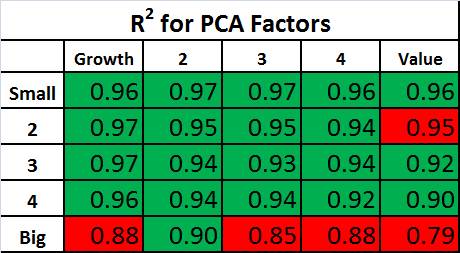
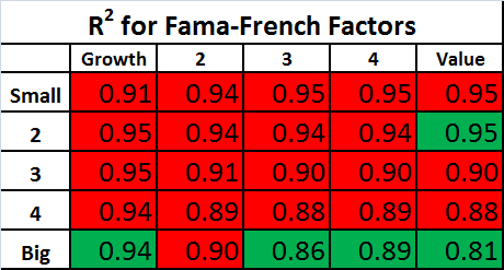
The R^2s are quite high using both sets of factors.  As expected, the R^2s are generally higher with the PCA factors, but the difference between the two factor models is small.

Similar tables are shown below for the alphas.  Keep in mind that the an effective factor model will have alphas that are close to zero, so for the tables below, the values are highlighted in green if the alpha is smaller in magnitude than the alternative model.

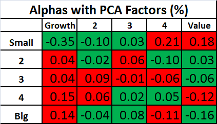
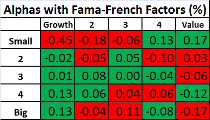
Again, the performance of the two models is remarkably similar!  This shows that the Fama-French factors are doing about as well in explaining these portfolios as is possible with three factors!

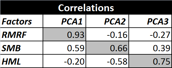
Correlation of PCA Factors and Fama-French Factors

Despite the similarity in R^2s and alphas, the two sets of factors do not, on initial inspection, show a lot of other close similarities beyond the first factor.  For example, the PCA factor loadings for the FF25 portfolios were plotted in the previous post, and they don’t look like we would expect the factor loadings to look for the Fama-French factors.

Also, if we look at the correlations between the two sets of factors, they aren’t particularly high for the 2nd and 3rd factors, although the first PCA factor, unsurprisingly, has a relatively high correlation to the market factor (RMRF).

Creating Synthetic Versions of RMRF, SMB, and HML

As mentioned in the previous post, the PCA factors have some interesting properties which don’t necessarily apply to real world sources of priced risk.  The PCA factors are uncorrelated, they are normalized, and they have the property that each in turn captures as much of the remaining variance as possible.

However, if we take linear combinations of the three PCA factors, we can preserve their ability to explain returns (the R^2 and Alpha are unchanged) while removing the other PCA related constraints. If we do this, it turns out that we can create factors which are nearly identical to the Fama-French factors.

I created the optimal linear combinations using Octave’s “ols” command.  For the specific procedure, see the script posted below.  I’m calling these new factors “synthetic” factors to distinguish them from the original Fama-French factors.  The correlations between the Fama-French factors and their synthetic equivalents are shown below.

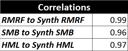
These correlations are quite high.  Perhaps this is not surprising since I fit the the PCA factors to the Fama-French factors, but I think it is important because it shows that there is very little covariance captured by the PCA factors which is not captured by the Fama-French factors.  In other works, the Fama-French three factor model is leaving almost nothing on the table when it comes to explaining the returns of the target portfolios.  The model does about as well as possible with three factors.

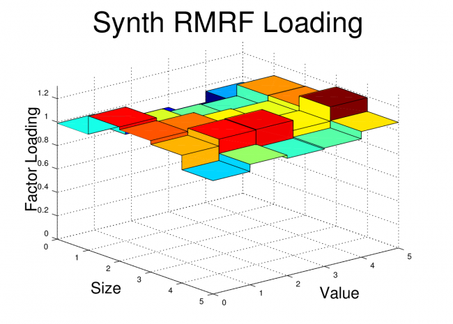
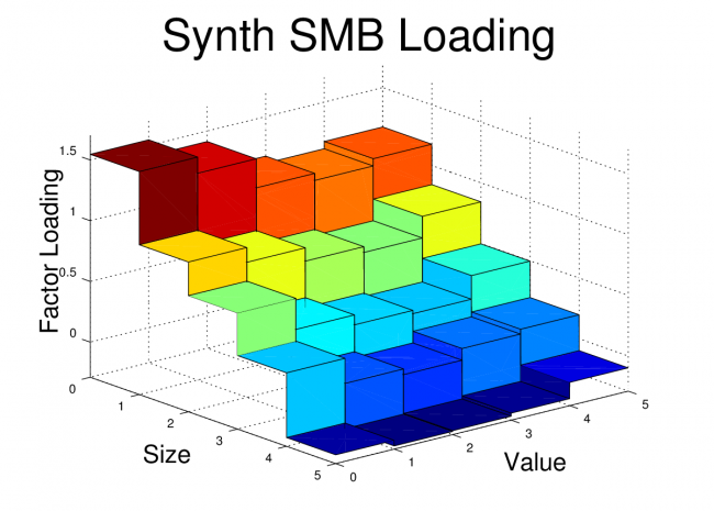
In order to drive this point home, I’ve also plotted the factor loadings of the FF25 portfolios for both the original Fama-French factors and the Synthetic Fama-French factors.  The corresponding plots look nearly identical.

Fama-French Factor Loadings 1962-2012

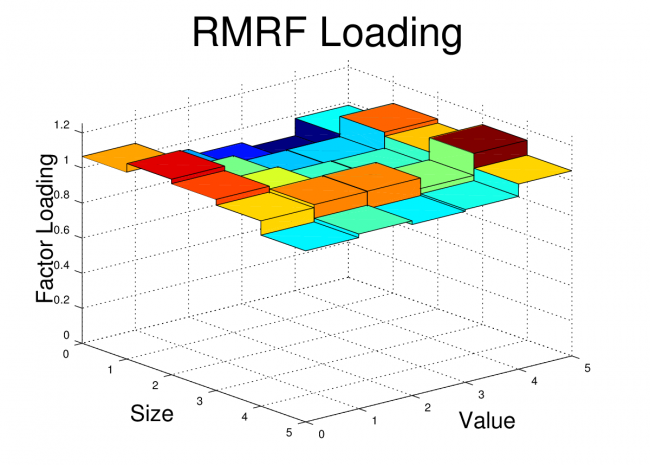
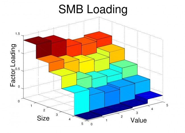
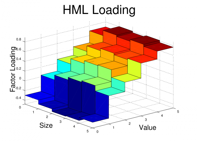
Synthetic Fama-French Factor Loadings 1962-2012

Conclusion

The goal of this post was to show that Fama and French’s simple method of forming long-short portfolios based on size and value sorts does a remarkably good job in producing factor portfolios which are nearly optimal for explaining a set of portfolios formed on size and value sorts.

For some readers, it may not be surprising to some that factors created using size and value do a good job of explaining portfolios which are sorted on size and value.  In fact, it may seem like a tautology.  However, the Fama-French factors have been shown to do quite well in explaining the returns of portfolios formed by a variety of other sorts, and it isn’t a given that portfolios should co-vary based on their size or value characteristic.

Code:

The Octave code to create the plots and tables is shown below.  The code for the “fivebyfive” function which is called by this script is provided in the previous post.

clear all;
close all;

% Load Portfolios and Factors
% First two files are from Kenneth French website (headers and other data removed)
% PCA file is generated from script used in previous post
ff_facts = load('F-F_Research_Data_Factors_monthly.txt');
ff_ports = load('25_Portfolios_5x5_monthly.txt');
pca_facts = load('pcafactors.txt');

% Determine Start and Stop points for FF factors
start_year = 1962;
start_month = 1;
stop_year = 2012;
stop_month = 12;

start = (start_year-1932)*12 + (start_month-1) + 67;
stop = (stop_year-1932)*12 + (stop_month-1) + 67;

% Grab FF factors over selected date range
rf = ff_facts(start:stop,5);
rmrf = ff_facts(start:stop,2);
smb = ff_facts(start:stop,3);
hml = ff_facts(start:stop,4);

% Grab PCA Factors (already starting at 1/1962)
pca1 = pca_facts(:,2);
pca2 = pca_facts(:,3);
pca3 = pca_facts(:,4);

% Grab portfolio data over selected range
x = ff_ports(start:stop,:); % start after NAs end i.e line 67
r = x(:,2:end);

% Excess returns of portfolios:
rx = r - repmat(rf,1,25);

% Correlations between Factors

corr(rmrf,pca1)
corr(rmrf,pca2)
corr(rmrf,pca3)

corr(smb,pca1)
corr(smb,pca2)
corr(smb,pca3)

corr(hml,pca1)
corr(hml,pca2)
corr(hml,pca3)

% Creating Synthetic RMRF, SMB, HML
rhv = [pca1 pca2 pca3];
[beta_rmrf] = ols(rmrf,rhv);
[beta_hml]=ols(hml,rhv);
[beta_smb] = ols(smb,rhv);

synth_rmrf = beta_rmrf(1)*pca1+beta_rmrf(2)*pca2+beta_rmrf(3)*pca3;
synth_hml = beta_hml(1)*pca1+beta_hml(2)*pca2+beta_hml(3)*pca3;
synth_smb = beta_smb(1)*pca1+beta_smb(2)*pca2+beta_smb(3)*pca3;

corr(rmrf,synth_rmrf)
corr(smb,synth_smb)
corr(hml,synth_hml)

%%%%%%%%%%%%%%%%%%%%%%%%%%%%%%%%%%%%%%%%%%%%%%%%%%%%%%%%%%%%%%%%%%%%
% Regress #1: Using Raw PCA Factors
%%%%%%%%%%%%%%%%%%%%%%%%%%%%%%%%%%%%%%%%%%%%%%%%%%%%%%%%%%%%%%%%%%%%
K=3
T=size(pca1,1);
rhv = [ones(T,1),pca1,pca2,pca3];
r_coefs = rhv\rx;

e = rx-rhv*r_coefs;
sigma = cov(e);
u = rx-rhv*r_coefs;
s2 = (T-1)/(T-K-1)*var(u)'; % NOTE var uses 1/T-1, I corrected to 1/T-K-1
R2_1 = 1-s2./(std(rx).^2)';
a_pca = r_coefs(1,:)';
b1_pca = r_coefs(2,:)';
b2_pca = r_coefs(3,:)';
b3_pca = r_coefs(4,:)';

%%%%%%%%%%%%%%%%%%%%%%%%%%%%%%%%%%%%%%%%%%%%%%%%%%%%%%%%%%%%%%%%%%%%
% Regress #2: Using FF Factors
%%%%%%%%%%%%%%%%%%%%%%%%%%%%%%%%%%%%%%%%%%%%%%%%%%%%%%%%%%%%%%%%%%%%

K=3;
T=size(rmrf,1);
rhv = [ones(T,1),rmrf,smb,hml];
r_coefs2 = rhv\rx;

e = rx-rhv*r_coefs;
sigma = cov(e);
u = rx-rhv*r_coefs2;
s2 = (T-1)/(T-K-1)*var(u)'; % Var uses 1/T-1, I corrected to 1/T-K-1
R2_2 = 1-s2./(std(rx).^2)';

% Extract Factor Loadings
a_ff = r_coefs2(1,:)';
b1_ff = r_coefs2(2,:)';
b2_ff = r_coefs2(3,:)';
b3_ff = r_coefs2(4,:)';

%%%%%%%%%%%%%%%%%%%%%%%%%%%%%%%%%%%%%%%%%%%%%%%%%%%%%%%%%%%%%%%%%%%
% Regress #3: Using Synthetic FF Factors
%%%%%%%%%%%%%%%%%%%%%%%%%%%%%%%%%%%%%%%%%%%%%%%%%%%%%%%%%%%%%%%%%%%
K=3;
T=size(rmrf,1);
rhv = [ones(T,1),synth_rmrf,synth_smb,synth_hml];
r_coefs3 = rhv\rx;

e = rx-rhv*r_coefs3;
sigma = cov(e);
u = rx-rhv*r_coefs3;
s2 = (T-1)/(T-K-1)*var(u)'; % Var uses 1/T-1, corrected to 1/T-K-1
R2_3 = 1-s2./(std(rx).^2)';

% Extract Factor Loadings
a_synth = r_coefs3(1,:)';
b1_synth = r_coefs3(2,:)';
b2_synth = r_coefs3(3,:)';
b3_synth = r_coefs3(4,:)';

%%%%%%%%%%%%%%%%%%%%%%%%%%%%%%%%%%%%%%%%%%%%%%%%%%%%%%%%%%%%%%%%%%%
% Compare Alphas and Rsq's
%%%%%%%%%%%%%%%%%%%%%%%%%%%%%%%%%%%%%%%%%%%%%%%%%%%%%%%%%%%%%%%%%%%

% Alphas for three sets of Factors
alpha1 = reshape(a_pca,5,5)
alpha2 = reshape(a_ff,5,5)
alpha3 = reshape(a_synth,5,5)

% R2 for three sets of Factors
rsq1 = reshape(R2_1,5,5)'  %R^2 for PCA factors
rsq2 = reshape(R2_2,5,5)'  %R^2 for Fama-French Factors
rsq3 = reshape(R2_3,5,5)'  %R^2 for Synthetic FF Factors

%%%%%%%%%%%%%%%%%%%%%%%%%%%%%%%%%%%%%%%%%%%%%%%%%%%%%%%%%%%%%%%%%%%
% Plot Factor Loads
%%%%%%%%%%%%%%%%%%%%%%%%%%%%%%%%%%%%%%%%%%%%%%%%%%%%%%%%%%%%%%%%%%%

figure;
fivebyfive(b1_ff);
xlabel('Size','fontsize',20)
ylabel('Value','fontsize',20)
zlabel('Factor Loading','rotation',90,'fontsize',20)
title('RMRF Loading','fontsize',36)
view(50,25)
print -dpng ff_rmrf.png

figure;
fivebyfive(b2_ff);
xlabel('Size','fontsize',20)
ylabel('Value','fontsize',20)
zlabel('Factor Loading','rotation',90,'fontsize',20)
title('SMB Loading','fontsize',36)
view(50,25)
print -dpng ff_smb.png

figure;
fivebyfive(b3_ff);
xlabel('Size','fontsize',20)
ylabel('Value','fontsize',20)
zlabel('Factor Loading','rotation',90,'fontsize',20)
title('HML Loading','fontsize',36)
view(50,25)
print -dpng ff_hml.png

figure;
fivebyfive(b1_synth);
xlabel('Size','fontsize',20)
ylabel('Value','fontsize',20)
zlabel('Factor Loading','rotation',90,'fontsize',20)
title('Synth RMRF Loading','fontsize',36)
view(50,25)
print -dpng synth_rmrf.png

figure;
fivebyfive(b2_synth);
xlabel('Size','fontsize',20)
ylabel('Value','fontsize',20)
zlabel('Factor Loading','rotation',90,'fontsize',20)
title('Synth SMB Loading','fontsize',36)
view(50,25)
print -dpng synth_smb.png

figure;
fivebyfive(b3_synth);
xlabel('Size','fontsize',20)
ylabel('Value','fontsize',20)
zlabel('Factor Loading','rotation',90,'fontsize',20)
title('Synth HML Loading','fontsize',36)
view(50,25)
print -dpng synth_hml.png