Calculating the Efficient Frontier with a Risk-Free Asset
So, I’ve been feeling a little bit bogged down on this efficient frontier topic, and I’m anxious to wrap things up with this post and move on to something more original!
In the previous two posts, I have demonstrated how to calculate the efficient frontier for any number of risky assets, and I’ve shown how to calculate the portfolio weights for each point on the efficient frontier.
In this post, I will conclude this series on the efficient frontier (finally!) by demonstrating how the frontier changes with the addition of a risk-free asset.
An example Octave script is provided for calculating and plotting the efficient frontier, capital allocation line, and tangency portfolio.
Tangency Portfolio with a Risk-Free Asset w/return R
The tangency portfolio is the intercept point if we draw a tangent line from the risk-free rate of return (on the y-axis) to the efficient frontier for risky assets.
The equations used to calculate the portfolio weights, expected return, and variance for the tangency portfolio are shown in this section.
The variables used in these equations are described in more detail in the previous posts. However, to review briefly, ![]() is the vector of expected returns for the risky assets, and
is the vector of expected returns for the risky assets, and ![]() is the covariance matrix for the returns of these assets. The values for A, B, C, and
is the covariance matrix for the returns of these assets. The values for A, B, C, and ![]() are intermediate values calculated using the portfolio statistics and the equations for these values are shown in my initial post on this topic. The value R is the return on the risk-free asset. The value
are intermediate values calculated using the portfolio statistics and the equations for these values are shown in my initial post on this topic. The value R is the return on the risk-free asset. The value ![]() is a vector showing the weight of each asset (weights sum to 1) in the tangency portfolio, and
is a vector showing the weight of each asset (weights sum to 1) in the tangency portfolio, and ![]() and
and ![]() are the expected return and variance of the tangency portfolio.
are the expected return and variance of the tangency portfolio.
![]()
![]()
![]()
Calculating a Point on the Capital Allocation Line
The Capital Allocation Line or CAL is the tangent line from the risk-free rate of return (on the y-axis) to the efficient frontier for risky assets. The points on this line represent the highest expected return we can get at a given level of risk when we have access to a risk-free asset.
All points on this line are a combination of the tangency portfolio and the risk-free asset. If the weight of the portfolio in the tangency portfolio is given as ![]() then the weight in the risk-free asset must be
then the weight in the risk-free asset must be ![]() . The value of
. The value of ![]() can be calculated for any desired expected return,
can be calculated for any desired expected return, ![]() on the CAL using this equation:
on the CAL using this equation:
![]()
Using this y-value we can calculate the standard deviation at this point on the CAL:
![]()
By combining these equations, we get the general equation for the CAL:
![]()
Example Calculation using Octave
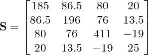
As an example, let’s consider the four risky assets used in the efficient frontier examples in the previous posts. The expected return vector and covariance matrix for these assets is given here:


The risk-free rate will be assumed to be 3%, and the target return will be set to 14%.
If we implement the equations for the tangency portfolio and CAL in Octave, we can calculate the portfolio weights for the tangency portfolio (![]() ), and the weight of the total portfolio which should be in the tangency portfolio (
), and the weight of the total portfolio which should be in the tangency portfolio (![]() ) and the risk-free asset (
) and the risk-free asset (![]() ) to achieve the target expected return.
) to achieve the target expected return.
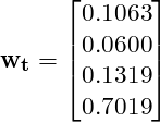
The portfolio weights for the tangency portfolio are shown here:

The weight in the tangency portfolio is:
![]()
Since this value is greater than 1, that means we have a short position in the risk-free asset with a weight of ![]() or -0.804.
or -0.804.
Note that this is a somewhat unrealistic scenario since we cannot borrow at the true risk-free rate. In practice our borrowing rate would be higher, and the actual risk-free rate would be used only for portfolios where we had a positive weight in the risk-free asset.
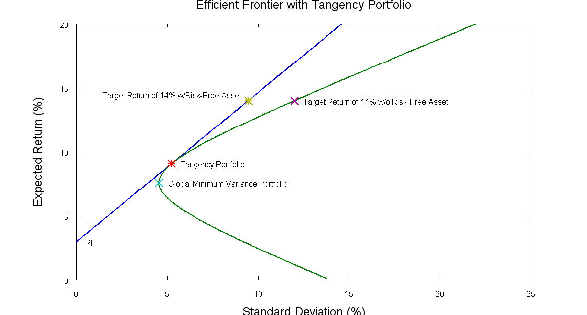
The plot of the efficient frontier, tangency portfolio, and the CAL are shown here:
Octave Code:
This Octave code will calculate and plot the efficient frontier, tangency portfolio and the CAL. The script can be modified for a different set of assets by updating the expected returns vector, the covariance matrix, the target return, and the risk free rate. The script will also work in Matlab.
clear all;
close all;

%%%%%%%%%%%%%%%%%%%%%%%%%%%%%%%%%%%%%%%%%%%%%%%%%%%%%%%%
% Mean Variance Optimizer Inputs
%%%%%%%%%%%%%%%%%%%%%%%%%%%%%%%%%%%%%%%%%%%%%%%%%%%%%%%%

% S is matrix of security covariances
S = [185 86.5 80 20; 86.5 196 76 13.5; 80 76 411 -19; 20 13.5 -19 25]

% Vector of security expected returns
zbar = [14; 12; 15; 7]

% Risk Free Asset Return
R = 3

% Target Return
mu_tar = 14

%%%%%%%%%%%%%%%%%%%%%%%%%%%%%%%%%%%%%%%%%%%%%%%%%%%%%%%
% Calculating Variables
%%%%%%%%%%%%%%%%%%%%%%%%%%%%%%%%%%%%%%%%%%%%%%%%%%%%%%%

% Unity vector..must have same length as zbar
unity = ones(length(zbar),1)

% Vector of security standard deviations
stdevs = sqrt(diag(S))

A = unity'*S^-1*unity
B = unity'*S^-1*zbar
C = zbar'*S^-1*zbar
D = A*C-B^2

% Calculate Lambda and Gamma
lambda_target = (C - mu_tar*B)/D;
gamma_target =  (mu_tar*A-B)/D;

%%%%%%%%%%%%%%%%%%%%%%%%%%%%%%%%%%%%%%%%%%%%%%%%%%%%%%%
% Efficient Frontier
%%%%%%%%%%%%%%%%%%%%%%%%%%%%%%%%%%%%%%%%%%%%%%%%%%%%%%%
mu = 1:200;
mu = mu/10;

minvar = ((A*mu.^2)-2*B*mu+C)/D;
minstd = sqrt(minvar);

plot(minstd,mu,stdevs,zbar,'*')
title('Efficient Frontier with Individual Securities','fontsize',18)
ylabel('Expected Return (%)','fontsize',18)
xlabel('Standard Deviation (%)','fontsize',18)

%%%%%%%%%%%%%%%%%%%%%%%%%%%%%%%%%%%%%%%%%%%%%%%%%%%%%%%
% Global Minimum Variance Portfolio
%%%%%%%%%%%%%%%%%%%%%%%%%%%%%%%%%%%%%%%%%%%%%%%%%%%%%%%

% Mean and Variance of Global Minimum Variance Portfolio
mu_g = B/A
var_g = 1/A
std_g = sqrt(var_g)

% Minimum Variance Portfolio Weights
w_g = (S^-1*unity)/A

%%%%%%%%%%%%%%%%%%%%%%%%%%%%%%%%%%%%%%%%%%%%%%%%%%%%%%%
% Tangency Portfolio with a Risk Free Asset
%%%%%%%%%%%%%%%%%%%%%%%%%%%%%%%%%%%%%%%%%%%%%%%%%%%%%%%

% Expected Return of Tangency Portfolio
ztan = (C-B*R)/(B-A*R);

% Variance and Standard Deviation of Tangency Portfolio
vartan = (C-2*R*B + R^2*A)/((B-A*R)^2);
stdtan = sqrt(vartan);

% Weights for Tangency Portfolio
w_tan = (S^-1*(zbar - R*unity))/(B-A*R)

% Tangency Line
mu_tan = mu(mu >= R);
minvar_rf = (mu_tan-R).^2/(C-2*R*B+A*R^2);
minstd_rf = sqrt(minvar_rf);

% Weights for w_d (tangency when R=0)
w_d = (S^-1*zbar)/B;

%%%%%%%%%%%%%%%%%%%%%%%%%%%%%%%%%%%%%%%%%%%%%%%%%%%%%%%
% Target Return Portfolio w/and w/o Risk Free Asset
%%%%%%%%%%%%%%%%%%%%%%%%%%%%%%%%%%%%%%%%%%%%%%%%%%%%%%%

% Weights for portfolio with target return = 14%, w/o risk-free asset

w_s = (lambda_target*A)*w_g + (gamma_target*B)*w_d;

% Expected Return of Target Portfolio (should match target)
mu_s = w_s'*zbar;

% Variance and Standard Deviation of target portfolio
var_s = w_s'*S*w_s;
std_s = sqrt(var_s);

% Weights for portfolio with target return = 14%, w/risk free asset

y = (mu_tar - R)/(ztan-R);
stdtar = stdtan*y;

%%%%%%%%%%%%%%%%%%%%%%%%%%%%%%%%%%%%%%%%%%%%%%%%%%%%%%%%
% Tangency Plot
%%%%%%%%%%%%%%%%%%%%%%%%%%%%%%%%%%%%%%%%%%%%%%%%%%%%%%%%

figure
plot(minstd_rf,'linewidth',2,mu_tan,minstd,'linewidth',2,mu,stdtan,ztan,'*','linewidth',2,std_g,mu_g,'x','linewidth',2,std_s,mu_s,'x','linewidth',2,stdtar,mu_tar,'*','linewidth',2)
text(0.5,R,'RF','fontsize',12);
text(0.5+std_g,mu_g,'Global Minimum Variance Portfolio','fontsize',12);
text(0.5+stdtan,ztan,'Tangency Portfolio','fontsize',12);
text(0.5+std_s,mu_s,'Target Return of 14% w/o Risk-Free Asset','fontsize',12);
text(stdtar-8,mu_tar+0.5,'Target Return of 14% w/Risk-Free Asset','fontsize',12);
title('Efficient Frontier with Tangency Portfolio','fontsize',18)
ylabel('Expected Return (%)','fontsize',18)
xlabel('Standard Deviation (%)','fontsize',18)


Hey CalcInv.
Fantastic article series. As Frontcon (MatLab) is not implemented in Octave, these pages has been great inspiration.
I have two questions. I would like to use this approach for a portfolio optimisation problem. But I need to evaluate on daily returns and stdev over daily returns (and in decimals instead of % – as in 0.10 instead of 10% etc.). I’m not sure how to do this trick. ( like transforming daily Sharpe to yearly with Yearly sharpe = Daily sharpe * sqrt(252)) – 252 trading days.
Also how do you add constraints, eg. no short positions (negative weight). ?
All the best!
Christian
Hi Christian,
As long as the horizon (daily, monthly, yearly, etc) is consistent for both the expected return vector and the covariance matrix the program should still work. You should be able to do this with daily returns without any changes, and it should work with decimals returns….again as long as everything is consistent.
The constraints problem is trickier. I don’t know of any non-iterative way to do the constrained optimization…i.e. I don’t think there is an easy modification you can make to the linear algebra equations. Instead I think you need to use some kind of iterative optimization technique.
-Chad
This looks very useful, thanks!
I seem to have a problem running this with my data, in particular I often get very small numbers in my covariance matrix (sometimes it’s singular) and the efficient frontier doesn’t look right.
If my assets are absolute weekly index prices am I correct in thinking that my expected returns are just the mean relative value of each index? E.g. I have zbar = [1.2; 13.51; 0.06; 0.88; 2.52]. And the covariance matrix is just cov(data) with data being the matrix of absolute prices, with each column being an asset, and each row a week? I’m not sure what I’m doing wrong, any help is appreciated.