My first post on this topic included R code for downloading monthly or weekly returns from Yahoo! Finance, and I created a short video tutorial to demonstrate the code. My second post provided a Google Docs spreadsheet which can be used to download monthly returns.

In this post, I’ve updated the original R code to allow monthly returns for multiple stocks or funds to be downloaded into a single CSV file. This is useful if you want to compare factor loadings for multiple funds, or if you simply want to get the monthly returns for all the funds in your portfolio.

The code uses an input file “funds.csv” which is a list of tickers symbols for the target stocks or funds.  An example file is available here.

The monthly returns are recorded in a file called “fundreturns.csv” which is stored in R’s working directory

Note that I believe Yahoo! Finance limits the amount of data that you can download from the site in a given period of time.  I don’t know the specific rules, but if you put a large number of tickers into the CSV file you might find that the downloads start failing and you’ll have to wait for some period of time before they start working again.

The R code is posted below.  The variable “startdate” should be set to a date a few days prior to the start of the first month for which you want to get return data.  For example, if the first monthly return you are targeting is January 2006, then you can set the start date to “12-25-2005”.  If the start date chosen is earlier than the earliest available price history for some funds, then there could be some misalignment between returns and dates in the output file, so be sure to choose a date which is compatible with available price history for the all the stocks and funds in your list.

R Code:

This code requires both the “tseries” and “zoo” packages to be installed.  For details on installing packages on your specific platform please see the R project documentation on package installation.

# Batch Fund Download
# calcinv: 09/19/2013

# Import tseries and zoo libraries
library(zoo)
library(tseries)

# Uncomment the setInternet2 line if a proxy is required
# setInternet2(TRUE)

# Set Start Date
startdate = "2005-12-25"

# Load CSV file into R
testfunds <- read.table("funds.csv",sep=";",header=FALSE)

# Extract tickers and fund weights
ticks <- testfunds[,1]

# Setup Equity Fund Variables
funds <- NULL

# Download equity fund data
for(i in 1:length(ticks)){
# Download Adjusted Price Series from Yahoo! Finance
prices <- get.hist.quote(ticks[i], quote="Adj", start=startdate, retclass="zoo")

# Convert daily closing prices to monthly closing prices
monthly.prices <- aggregate(prices, as.yearmon, tail, 1)

# Convert selected monthly prices into monthly returns to run regression
r <- diff(log(monthly.prices))  # convert prices to log returns
r1 <- exp(r)-1                  # back to simple returns

# Now shift out of zoo object into ordinary matrix
rj <- coredata(r1)

# Put fund returns into matrix
funds <- cbind(funds, rj)
}

fundfile <- cbind(as.character(index(r1)),funds)
header <- c("Dates",as.character(ticks))
fundfile <- rbind(header,fundfile)

# Write output data to csv file
write.table(fundfile, file="fundreturns.csv", sep=",", row.names=FALSE,col.names=FALSE)

The plots below show the housing price history for major cities within each region. Each plot also includes the 20 city average data series.  Each city’s price history is normalized to 100 in January 2000.  Since the Case-Shiller data is not adjusted for inflation, I also added a normalized CPI-U series to each plot.

The “Mortgage Payment” plot shows the price indices adjusted to account for changing mortgage rates.  This plot incorporates both the Case-Shiller data and the mortgage rate to show how the payments for a 30 year fixed rate mortgage have varied for a “constant-quality” home.

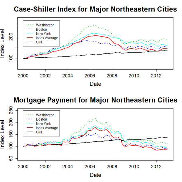
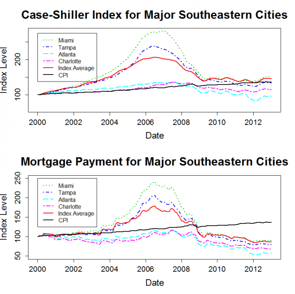
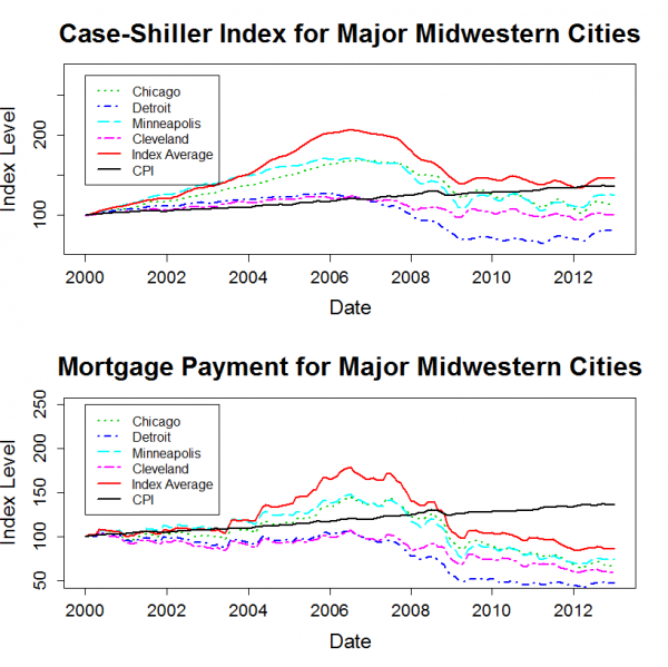
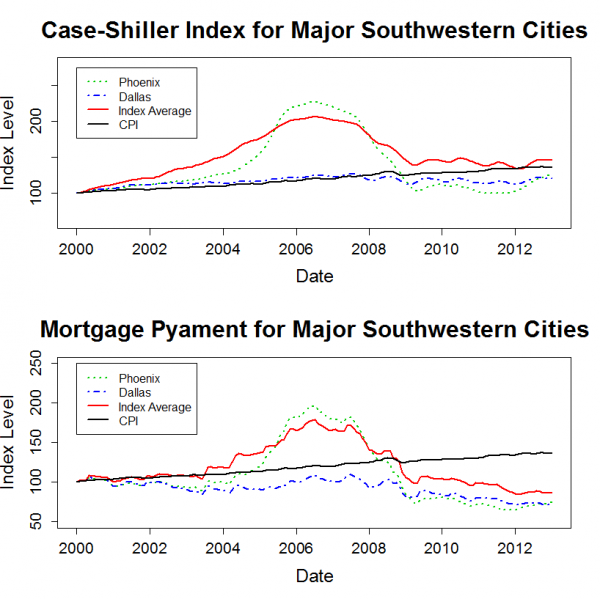
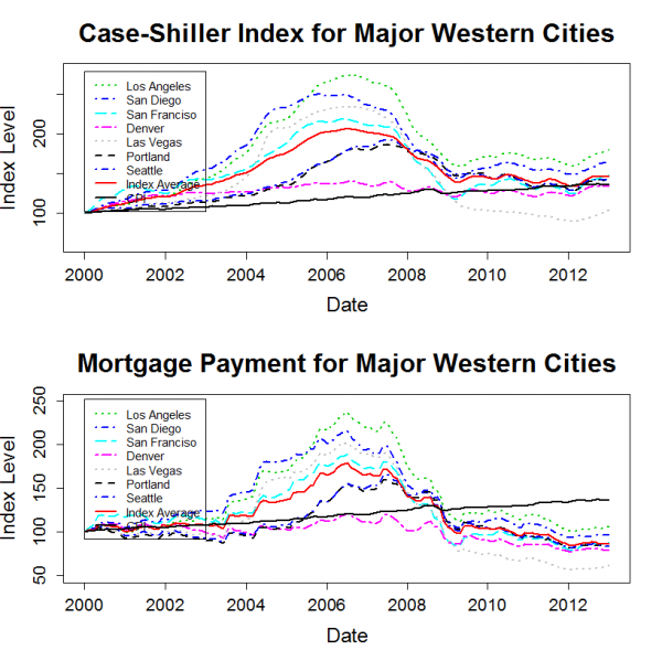
Takeaways

The plots show that, for most markets, nominal home prices have leveled out over the past two years.  However, mortgage rates have continued to decline a bit, so the total cost for new home buyers with a 30-year mortgage has continued to trend downwards.

Home prices in many markets are lower in real terms than they were in 2000.  The west and the northeast are the exceptions.  Despite severe declines from bubble highs, prices in these regions have generally risen by more than inflation since 2000.

R Code:

The R code for generating these plots and specifics of the mortgage payment calculation are given in the original post.

The goal of this post is to determine whether or not the Fama-French factors are leaving anything significant on the table that the PCA factors, which capture as much covariance in the target portfolios as is possible with three factors, are able to pick up.

In other words, I’ll be comparing the R^2s and alphas for both the Fama-French factors and the PCA factors, and, after some re-arranging, I’ll also compare the factor loadings.

Data

The Fama-French 3 Factor (FF3F) data and the Fama-French 25 size and value sorted portfolio (FF25) data come from the Kenneth French website.  The PCA factors were calculated in the previous post, and I posted the data in a Google Docs Spreadsheet.

R^2 and Alpha using PCA Factors and Fama French Factors

As a first step, the R^2s and alphas for the FF25 portfolios can be calculated using both the Fama-French factors and the PCA factors.

The PCA factors will give us the best fit across the 25 portfolios that is possible with three factors, so we expect the R^2s for the Fama-French factors to be lower on average. The question is: How much lower?

The tables below show the R^2s for the PCA Factors and Fama-French Factors.  For each table, the values highlighted in green have an R^2 which is higher than the alternative model, and the values highlighted in red have an R^2 which is lower than the alternative model.

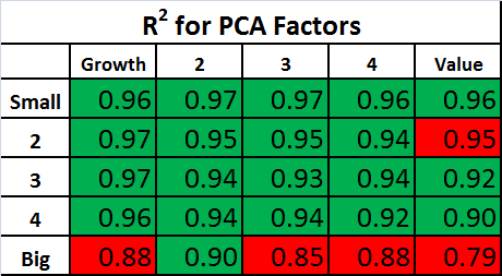
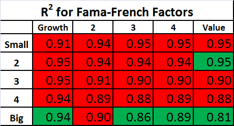
The R^2s are quite high using both sets of factors.  As expected, the R^2s are generally higher with the PCA factors, but the difference between the two factor models is small.

Similar tables are shown below for the alphas.  Keep in mind that the an effective factor model will have alphas that are close to zero, so for the tables below, the values are highlighted in green if the alpha is smaller in magnitude than the alternative model.

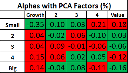
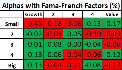
Again, the performance of the two models is remarkably similar!  This shows that the Fama-French factors are doing about as well in explaining these portfolios as is possible with three factors!

Correlation of PCA Factors and Fama-French Factors

Despite the similarity in R^2s and alphas, the two sets of factors do not, on initial inspection, show a lot of other close similarities beyond the first factor.  For example, the PCA factor loadings for the FF25 portfolios were plotted in the previous post, and they don’t look like we would expect the factor loadings to look for the Fama-French factors.

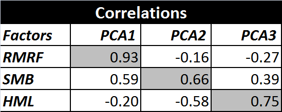
Also, if we look at the correlations between the two sets of factors, they aren’t particularly high for the 2nd and 3rd factors, although the first PCA factor, unsurprisingly, has a relatively high correlation to the market factor (RMRF).

Creating Synthetic Versions of RMRF, SMB, and HML

As mentioned in the previous post, the PCA factors have some interesting properties which don’t necessarily apply to real world sources of priced risk.  The PCA factors are uncorrelated, they are normalized, and they have the property that each in turn captures as much of the remaining variance as possible.

However, if we take linear combinations of the three PCA factors, we can preserve their ability to explain returns (the R^2 and Alpha are unchanged) while removing the other PCA related constraints. If we do this, it turns out that we can create factors which are nearly identical to the Fama-French factors.

I created the optimal linear combinations using Octave’s “ols” command.  For the specific procedure, see the script posted below.  I’m calling these new factors “synthetic” factors to distinguish them from the original Fama-French factors.  The correlations between the Fama-French factors and their synthetic equivalents are shown below.

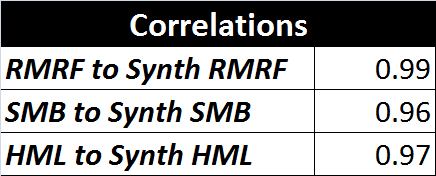
These correlations are quite high.  Perhaps this is not surprising since I fit the the PCA factors to the Fama-French factors, but I think it is important because it shows that there is very little covariance captured by the PCA factors which is not captured by the Fama-French factors.  In other works, the Fama-French three factor model is leaving almost nothing on the table when it comes to explaining the returns of the target portfolios.  The model does about as well as possible with three factors.

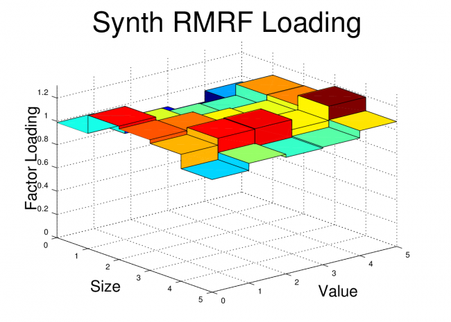
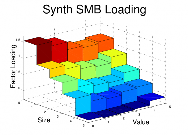
In order to drive this point home, I’ve also plotted the factor loadings of the FF25 portfolios for both the original Fama-French factors and the Synthetic Fama-French factors.  The corresponding plots look nearly identical.

Fama-French Factor Loadings 1962-2012

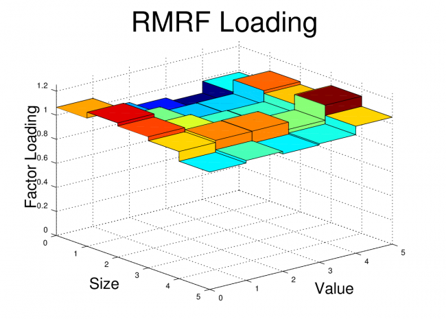
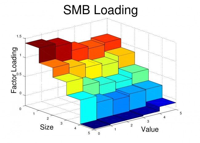
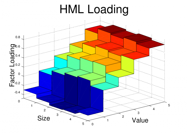
Synthetic Fama-French Factor Loadings 1962-2012

Conclusion

The goal of this post was to show that Fama and French’s simple method of forming long-short portfolios based on size and value sorts does a remarkably good job in producing factor portfolios which are nearly optimal for explaining a set of portfolios formed on size and value sorts.

For some readers, it may not be surprising to some that factors created using size and value do a good job of explaining portfolios which are sorted on size and value.  In fact, it may seem like a tautology.  However, the Fama-French factors have been shown to do quite well in explaining the returns of portfolios formed by a variety of other sorts, and it isn’t a given that portfolios should co-vary based on their size or value characteristic.

Code:

The Octave code to create the plots and tables is shown below.  The code for the “fivebyfive” function which is called by this script is provided in the previous post.

clear all;
close all;

% Load Portfolios and Factors
% First two files are from Kenneth French website (headers and other data removed)
% PCA file is generated from script used in previous post
ff_facts = load('F-F_Research_Data_Factors_monthly.txt');
ff_ports = load('25_Portfolios_5x5_monthly.txt');
pca_facts = load('pcafactors.txt');

% Determine Start and Stop points for FF factors
start_year = 1962;
start_month = 1;
stop_year = 2012;
stop_month = 12;

start = (start_year-1932)*12 + (start_month-1) + 67;
stop = (stop_year-1932)*12 + (stop_month-1) + 67;

% Grab FF factors over selected date range
rf = ff_facts(start:stop,5);
rmrf = ff_facts(start:stop,2);
smb = ff_facts(start:stop,3);
hml = ff_facts(start:stop,4);

% Grab PCA Factors (already starting at 1/1962)
pca1 = pca_facts(:,2);
pca2 = pca_facts(:,3);
pca3 = pca_facts(:,4);

% Grab portfolio data over selected range
x = ff_ports(start:stop,:); % start after NAs end i.e line 67
r = x(:,2:end);

% Excess returns of portfolios:
rx = r - repmat(rf,1,25);

% Correlations between Factors

corr(rmrf,pca1)
corr(rmrf,pca2)
corr(rmrf,pca3)

corr(smb,pca1)
corr(smb,pca2)
corr(smb,pca3)

corr(hml,pca1)
corr(hml,pca2)
corr(hml,pca3)

% Creating Synthetic RMRF, SMB, HML
rhv = [pca1 pca2 pca3];
[beta_rmrf] = ols(rmrf,rhv);
[beta_hml]=ols(hml,rhv);
[beta_smb] = ols(smb,rhv);

synth_rmrf = beta_rmrf(1)*pca1+beta_rmrf(2)*pca2+beta_rmrf(3)*pca3;
synth_hml = beta_hml(1)*pca1+beta_hml(2)*pca2+beta_hml(3)*pca3;
synth_smb = beta_smb(1)*pca1+beta_smb(2)*pca2+beta_smb(3)*pca3;

corr(rmrf,synth_rmrf)
corr(smb,synth_smb)
corr(hml,synth_hml)

%%%%%%%%%%%%%%%%%%%%%%%%%%%%%%%%%%%%%%%%%%%%%%%%%%%%%%%%%%%%%%%%%%%%
% Regress #1: Using Raw PCA Factors
%%%%%%%%%%%%%%%%%%%%%%%%%%%%%%%%%%%%%%%%%%%%%%%%%%%%%%%%%%%%%%%%%%%%
K=3
T=size(pca1,1);
rhv = [ones(T,1),pca1,pca2,pca3];
r_coefs = rhv\rx;

e = rx-rhv*r_coefs;
sigma = cov(e);
u = rx-rhv*r_coefs;
s2 = (T-1)/(T-K-1)*var(u)'; % NOTE var uses 1/T-1, I corrected to 1/T-K-1
R2_1 = 1-s2./(std(rx).^2)';
a_pca = r_coefs(1,:)';
b1_pca = r_coefs(2,:)';
b2_pca = r_coefs(3,:)';
b3_pca = r_coefs(4,:)';

%%%%%%%%%%%%%%%%%%%%%%%%%%%%%%%%%%%%%%%%%%%%%%%%%%%%%%%%%%%%%%%%%%%%
% Regress #2: Using FF Factors
%%%%%%%%%%%%%%%%%%%%%%%%%%%%%%%%%%%%%%%%%%%%%%%%%%%%%%%%%%%%%%%%%%%%

K=3;
T=size(rmrf,1);
rhv = [ones(T,1),rmrf,smb,hml];
r_coefs2 = rhv\rx;

e = rx-rhv*r_coefs;
sigma = cov(e);
u = rx-rhv*r_coefs2;
s2 = (T-1)/(T-K-1)*var(u)'; % Var uses 1/T-1, I corrected to 1/T-K-1
R2_2 = 1-s2./(std(rx).^2)';

% Extract Factor Loadings
a_ff = r_coefs2(1,:)';
b1_ff = r_coefs2(2,:)';
b2_ff = r_coefs2(3,:)';
b3_ff = r_coefs2(4,:)';

%%%%%%%%%%%%%%%%%%%%%%%%%%%%%%%%%%%%%%%%%%%%%%%%%%%%%%%%%%%%%%%%%%%
% Regress #3: Using Synthetic FF Factors
%%%%%%%%%%%%%%%%%%%%%%%%%%%%%%%%%%%%%%%%%%%%%%%%%%%%%%%%%%%%%%%%%%%
K=3;
T=size(rmrf,1);
rhv = [ones(T,1),synth_rmrf,synth_smb,synth_hml];
r_coefs3 = rhv\rx;

e = rx-rhv*r_coefs3;
sigma = cov(e);
u = rx-rhv*r_coefs3;
s2 = (T-1)/(T-K-1)*var(u)'; % Var uses 1/T-1, corrected to 1/T-K-1
R2_3 = 1-s2./(std(rx).^2)';

% Extract Factor Loadings
a_synth = r_coefs3(1,:)';
b1_synth = r_coefs3(2,:)';
b2_synth = r_coefs3(3,:)';
b3_synth = r_coefs3(4,:)';

%%%%%%%%%%%%%%%%%%%%%%%%%%%%%%%%%%%%%%%%%%%%%%%%%%%%%%%%%%%%%%%%%%%
% Compare Alphas and Rsq's
%%%%%%%%%%%%%%%%%%%%%%%%%%%%%%%%%%%%%%%%%%%%%%%%%%%%%%%%%%%%%%%%%%%

% Alphas for three sets of Factors
alpha1 = reshape(a_pca,5,5)
alpha2 = reshape(a_ff,5,5)
alpha3 = reshape(a_synth,5,5)

% R2 for three sets of Factors
rsq1 = reshape(R2_1,5,5)'  %R^2 for PCA factors
rsq2 = reshape(R2_2,5,5)'  %R^2 for Fama-French Factors
rsq3 = reshape(R2_3,5,5)'  %R^2 for Synthetic FF Factors

%%%%%%%%%%%%%%%%%%%%%%%%%%%%%%%%%%%%%%%%%%%%%%%%%%%%%%%%%%%%%%%%%%%
% Plot Factor Loads
%%%%%%%%%%%%%%%%%%%%%%%%%%%%%%%%%%%%%%%%%%%%%%%%%%%%%%%%%%%%%%%%%%%

figure;
fivebyfive(b1_ff);
xlabel('Size','fontsize',20)
ylabel('Value','fontsize',20)
zlabel('Factor Loading','rotation',90,'fontsize',20)
title('RMRF Loading','fontsize',36)
view(50,25)
print -dpng ff_rmrf.png

figure;
fivebyfive(b2_ff);
xlabel('Size','fontsize',20)
ylabel('Value','fontsize',20)
zlabel('Factor Loading','rotation',90,'fontsize',20)
title('SMB Loading','fontsize',36)
view(50,25)
print -dpng ff_smb.png

figure;
fivebyfive(b3_ff);
xlabel('Size','fontsize',20)
ylabel('Value','fontsize',20)
zlabel('Factor Loading','rotation',90,'fontsize',20)
title('HML Loading','fontsize',36)
view(50,25)
print -dpng ff_hml.png

figure;
fivebyfive(b1_synth);
xlabel('Size','fontsize',20)
ylabel('Value','fontsize',20)
zlabel('Factor Loading','rotation',90,'fontsize',20)
title('Synth RMRF Loading','fontsize',36)
view(50,25)
print -dpng synth_rmrf.png

figure;
fivebyfive(b2_synth);
xlabel('Size','fontsize',20)
ylabel('Value','fontsize',20)
zlabel('Factor Loading','rotation',90,'fontsize',20)
title('Synth SMB Loading','fontsize',36)
view(50,25)
print -dpng synth_smb.png

figure;
fivebyfive(b3_synth);
xlabel('Size','fontsize',20)
ylabel('Value','fontsize',20)
zlabel('Factor Loading','rotation',90,'fontsize',20)
title('Synth HML Loading','fontsize',36)
view(50,25)
print -dpng synth_hml.png

The three factors can be used to explain, though not predict, the returns for a variety of diversified portfolios. Many posts on this blog use the Fama-French 3 Factor (FF3F) model, including a tutorial on running the 3-factor regression using R.

An alternative way to construct factors is to use linear algebra to create “optimal” factors using a technique such as principal component analysis (PCA). This post will show how to construct the statistically optimal factors for the Fama-French 25 portfolios (sorted by size and value).

In my next post, I will compare these PCA factors to the Fama-French factors.

Description of Data

The data used for this analysis comes from the Kenneth French website.  I’m using the Fama-French 25 (FF25) portfolio returns which are available in the file titled “25 Portfolios Formed on Size and Book-to-Market”.  I’m using the returns from 1962 through 2012 since the pre-Compustat era portfolios have relatively few stocks.

The Fama-French factors are also available on the Kenneth French website in the file titled “Fama/French Factors”.  In this post, I will use not use the Fama-French factors themselves, but I do use the factor data file to get the monthly risk-free rate.

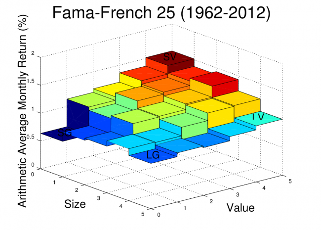
For reference, the arithmetic average monthly returns of the FF25 portfolios are plotted for the date range used in this analysis.  The Octave script to create this plot was provided in an earlier post.

Principal Component Analysis Example

PCA is a method for constructing factors which are uncorrelated with each other and which allow us to maximize R^2 when running regressions on the target portfolios. We can find the PCA factors with just a few lines of Octave code!

Step 1: Construct a matrix of excess returns

If we have a set of portfolios, we can show the returns in a matrix where each column is a portfolio and each row is a return.

For example, if I have 25 portfolios with 612 months of return data, I can structure these returns in a 612 by 25 matrix, where the first row is the earliest return for each portfolio.  Generally, when working with equity return factor models, the monthly risk-free rate is deducted from each monthly return, so the returns used are excess returns.

For this example, I have “preassembled” the excess return matrix and I read it in from a text file with the following Octave command:

rx = load(‘excessreturns.txt’)

Step 2: Calculate the Covariance Matrix

The Octave function “cov” can be used to calculate the covariance matrix for our return data.

Sigma_rx=cov(rx)

Step 3: Calculate the Eigenvalue Decomposition

Once we have the covariance matrix, we can use Octave to find the eigenvalue decomposition using the “eig” function:

[V,Lambda]=eig(Sigma)

The V columns are the eigenvectors and the diagonal elements of Lambda are the eigenvalues.

Step 4: Sort by Largest Standard Deviation and Extract Factor Loads

We need to sort the eigenvalues so that we can determine which factors will capture the highest variance of the data, so we first pull out the diagonal elements of Lambda and sort from largest to smallest.  This sort order is then applied to the eigenvectors.

[stdevs,order]=sort(diag(Lambda)’.^0.5,’descend’)

V = V(:,order)

Note that I’m taking the square root, so the variances become standard deviations.  This step is not necessary, but I like to look at the standard deviations rather than the variances when plotting.  The standard deviations for each vector can be plotted using the “bar” command.

bar(stdevs)

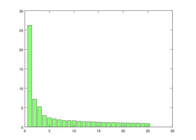
You can see that standard deviation captured by each additional factor trails off rapidly.  So, for this analysis, I’m just going to use the first three factors.

Step 5: Calculate the PCA Factors

The columns of V are the eigenvectors, and we sorted V so the eigenvectors accounting for the greatest variance in the data are ordered first.  Since the eigenvector column can be interpreted as a factor load for each of our original portfolios, we can create the factors themselves with a matrix multiplication.  Note that I don’t “center” the matrix rx, which is usually done for PCA.  In this case, I want to retain the mean because these new factors are essentially portfolio returns, and I want to be able to get meaningful alphas when I use them in regressions.

factors = rx*V

The first three factors that we are interested in will be the first three columns of the new factors matrix.

f1 = factors(:,1)
f2 = factors(:,2)
f3 = factors(:,3)

We now have our three PCA factors!

Example Code (Simple Version):

rx = load('excessreturns.txt');                        % Load Excess Returns
Sigma_rx = cov(rx);                                    % Calculate covariance matrix of excess returns</em>
[V,Lambda]=eig(Sigma_rx);                              % Eigenvalue decomposition
[stdevs,order] = sort(diag(Lambda)'.^0.5,'descend');   % Sort standard deviations in decending order
bar(stdevs)                                            % Plot standard deviations to see importance of each factor
V = V(:,order);                                        % Sort Eigenvectors in similar way
factors = rx*V;                                        % Calculate Factors
f1 = factors(:,1);                                     % Extract Factor 1
f2 = factors(:,2);                                     % Extract Factor 2
f3 = factors(:,3);                                     % Extract Factor 3

The First Three PCA Factors and Factor Loads for the FF25

The first three PCA factors generated by the script above can be used to analyze portfolios  in a manner similar to the Fama-French factors.  However, unlike the Fama-French factors, the PCA factors do not have a simple interpretation such as “size” or “value”.  Nevertheless, Arbitrage Pricing Theory suggests that we should see small alphas if the R^2 for the regression is high.

For reference, I’ve posted the three PCA equity factors in a Google Docs Spreadsheet. It is an interesting exercise to run some regressions using these factors and to compare the results with the FF3F model. The PCA factors should be expected to give higher R^2 for the FF25 portfolios since they are optimized to fit that data, but the results could be better or worse when tested on other types of portfolios.

For the FF25 portfolios, we don’t need to run any regressions to get the factor loads. The factor loads for each PCA factor are simply the corresponding columns of V.

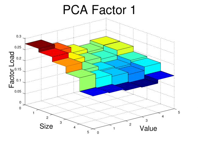
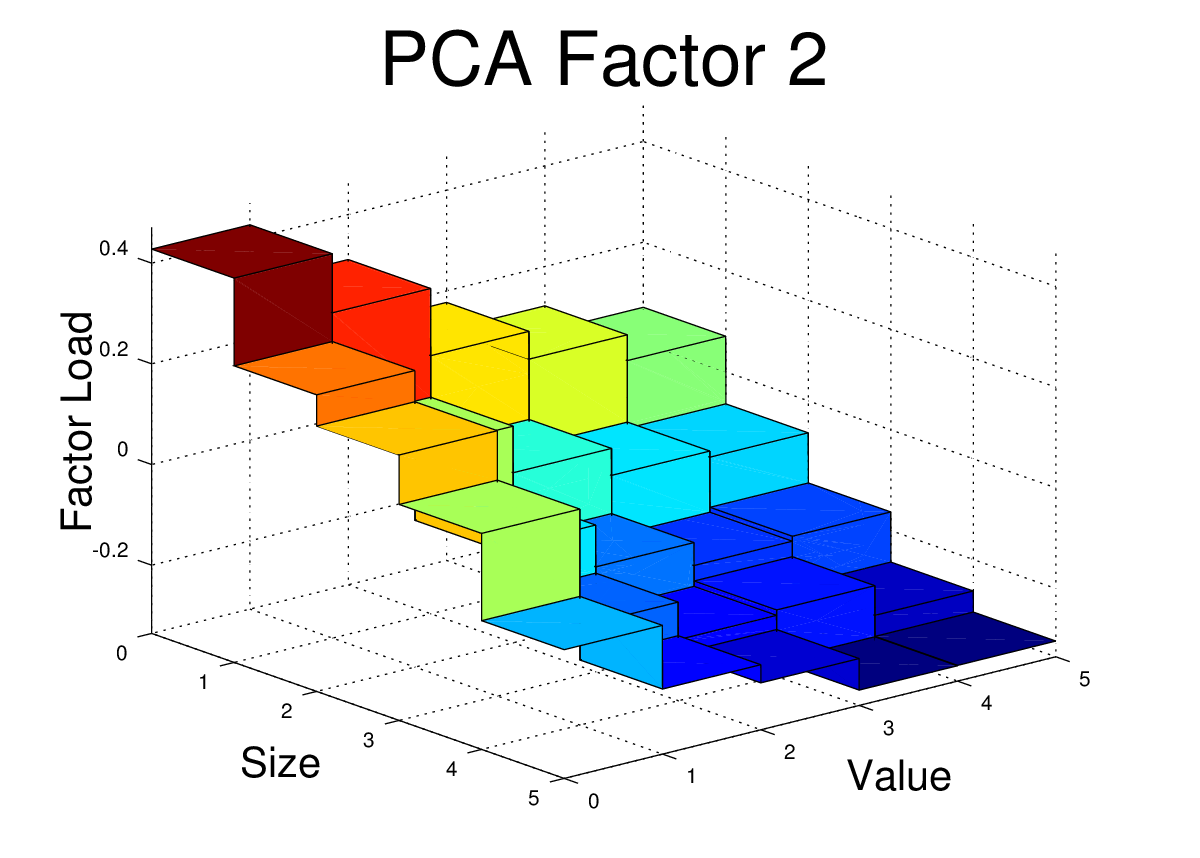
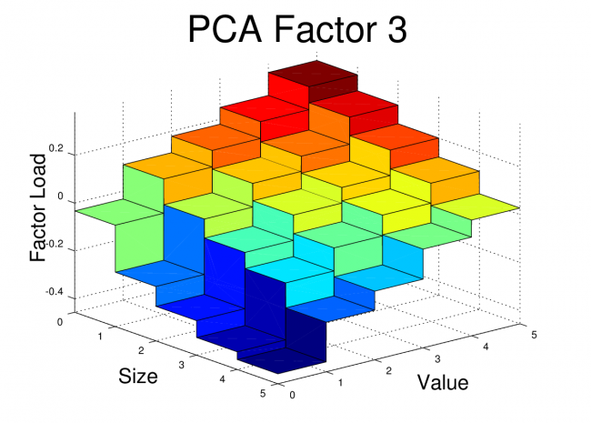
I’ve plotted the FF25 factor loads for the first three PCA equity factors here.  The code to generate these plots is shown at the end of this post.

Conclusion

At first glance, these PCA factor loads for the FF25 don’t bear much resemblance to what we would see with the FF3F model. For example, we would expect HML to have a loading which was relatively flat along the size axis, but which increased as we moved towards higher “value”. We would expect SMB loadings to be relatively flat across the value dimension, but to step up as we moved towards smaller size.

However, the PCA factors have certain properties that real world risk factors won’t necessarily have. The PCA factors are uncorrelated, they are normalized, and each in turn captures as much of the remaining covariance as possible. So, even if the PCA is successfully picking up covariance caused by real risk there may be equally effective factors (effective in terms of getting low alpha and high R^2) which are  linear combinations of these PCA factors. In fact, some linear combination of these three factors may give use something very similar to the FF3F factors.  In the next post, I’ll dig into this idea further.

Example Code (Extended Version):

Main Script:

clear all;
close all;

% Load Factors and Portfolio Returns
% The target files are the files from the Kenneth French website with comment text and data other than monthly returns

removed.
ff_facts = load('F-F_Research_Data_Factors_monthly.txt');
ff_ports = load('25_Portfolios_5x5_monthly.txt');

% Determine Start and Stop points for FF factors
% 1962 chosen so that only Compustat era data is used
start_year = 1962;
start_month = 1;
stop_year = 2012;
stop_month = 12;
start = (start_year-1932)*12 + (start_month-1) + 67;
stop = (stop_year-1932)*12 + (stop_month-1) + 67;

% Pullout risk free rate starting on start date
rf = ff_facts(start:stop,5);

% Pull out FF25 Portfolio Returns for Specified Date Range
x = ff_ports(start:stop,:); % start after NAs end i.e line 67
r = x(:,2:end);             % remove first column which is dates
rx = r - repmat(rf,1,25);   % calculate excess returns for portfolios

Sigma_rx = cov(rx);                                   % Calculate covariance matrix of excess returns
[V,Lambda]=eig(Sigma_rx);                             % Eigenvalue decomposition
[stdevs,order] = sort(diag(Lambda)'.^0.5,'descend');  % Sort standard deviations in decending order
bar(stdevs)                                           % Plot standard deviations to see importance of each factor
print -dpng scree.png                                 % Print to file
V = V(:,order);                                       % Sort Eigenvectors in similar way
factors = rx*V;                                       % Calculate Factors
f1 = factors(:,1);                                    % Extract Factor 1
f2 = factors(:,2);                                    % Extract Factor 2
f3 = factors(:,3);                                    % Extract Factor 3

% Create 3-D Plots of Factor Loadings (Columns of V)

figure;
fivebyfive(V(:,1));
xlabel('Size','fontsize',20)
ylabel('Value','fontsize',20)
zlabel('Factor Load','rotation',90,'fontsize',20)
title('PCA Factor 1','fontsize',36)
view(50,25)
print -dpng pca1.png

figure;
fivebyfive(V(:,2));
xlabel('Size','fontsize',20)
ylabel('Value','fontsize',20)
zlabel('Factor Load','rotation',90,'fontsize',20)
title('PCA Factor 2','fontsize',36)
view(50,25)
print -dpng pca2.png

figure;
fivebyfive(V(:,3));
xlabel('Size','fontsize',20)
ylabel('Value','fontsize',20)
zlabel('Factor Load','rotation',90,'fontsize',20)
title('PCA Factor 3','fontsize',36)
view(50,25)
print -dpng pca3.png

% Write Factors to file
dates = x(:,1);
pcafactors = [dates f1 f2 f3 rf];
save -ascii pcafactors.txt pcafactors

Function used by main script. This script should be saved in the working directory as “fivebyfive.m”.

function[] = fivebyfive(zvalues);

% Expand 5x5 data to 10x10 for use in surface plot function
zvals = [zvalues' ; zvalues'];
zvals = reshape(zvals,10,5);
zvals = [zvals;zvals];
zvals = reshape(zvals,10,10);

% Define x and y values
x = [0 0.999 1 1.999 2 2.999 3 3.999 4 5];
y = [0 0.999 1 1.999 2 2.999 3 3.999 4 5];

% Create x-y mesh for surface plot
[xx,yy] = meshgrid(x,y);

% Generate Plot
surf(xx,yy,zvals)
xlabel('Size','fontsize',20)
ylabel('Value','fontsize',20)
zlabel('Factor Load','rotation',90,'fontsize',20)
axis([0 5 0 5 min(0,min(zvalues)-0.1*abs(min(zvalues))) max(zvalues)+0.1*abs(max(zvalues))])

Have you ever wondered how much the level of the stock market can vary over one week?  What about two weeks or a month?

Until recently, I had not thought much about the range of short term market fluctuations. After all, I consider myself a long-term investor! However, a recent experience piqued my curiosity, and I decided to do a little research.

About a month ago, I transferred a small retirement account from a former employer into another existing retirement account.  I wasn’t able to do an electronic transaction or a “transfer in-kind“, so  I had to liquidate the old account before sending the funds to the new account provider.  The provider of the old account issued a paper check, and there was a surprisingly long delay for mailing and processing before the funds showed up in the new account.

The experience got me thinking about the risk of being out of the market (in cash) for short periods of time while transferring funds between accounts. The market may fall (good!) or rise (bad!) by a meaningful amount in a fairly short time.  If the amount being transferred is large, the risk can be significant.

In this post, I’ll look at some historical statistics on short term market returns.

Data Source and Methodology

I downloaded daily return data from July 1963 – August 2012 from the Ken French website.  The returns are available in the Fama/French Factors [Daily] file.  The daily risk-free rate needs to be added back into the RMRF column to get the total returns.  Note that these are “total stock market” returns, so the results may differ slightly from a similar analysis using S&P500 returns.

I calculated compound returns over rolling periods of 5, 10, 15, and 20 trading days.  I did not restrict the analysis to calendar week boundaries.  I then calculated a number of statistics on the 1, 5, 10, 15, and 20 day returns.

Note that the short-term return distributions are very “fat-tailed”, so I didn’t do any statistics which assume normal distribution.  Instead, I calculated the historical frequency of returns which exceed the various cutoffs.

Summary Statistics

Conclusions

The market can be extremely volatile over short time periods!  This creates a big risk if you must be out of the market for a couple weeks while transferring money between accounts.

For example, assume you transfer $100,000 and the transfer takes 10 days to complete.  You are out of the market for the full 10 days.  Historically, investors have, on average, missed out of $420 of gains over a 10 day period ($100,000 x 0.42%).  The median outcome is that you will miss out of $690 of gains ($100,000 x 0.69%).  Of course, there has also been a 4.6% possibility that the market will fall by 5% or more, and you will end up more than $5000 ahead!

My takeaway from this analysis is that transfers of funds which cannot be done electronically or in-kind should be planned carefully and monitored closely to ensure minimal delay.

A frequent debate among index fund investors involves “tilting” or over-weighting particular asset classes.  Usually, the asset classes to be over-weighted are small cap and value stocks.

Some investors believe that a portfolio tilted towards small cap and value is superior to a market-weight portfolio.  These investors believe that over-weighting these asset classes (relative to market-weight) and under-weighting other asset classes increases the likelihood of a superior outcome ( i.e. higher returns, lower risk, or both).

Other investors believe that a market-weight or TSM (Total Stock Market) portfolio is the best choice.  These investors believe we don’t know which asset classes are most likely to outperform in the future, and that the market weights reflect the best balance of risk and reward given the information available to investors at any particular time.

Debates often involve detailed analysis of past performance which, of course, has only limited value for forecasting the future!

Nevertheless, even making apples-to-apples comparisons of past performance is complicated because “live” index funds which track the various asset classes have been available for a relatively short time.

Academic datasets for TSM, small cap, and value indexes exist for longer periods of time (back to 1926 for U.S. stocks), but these indexes do not account for fund expenses and trading costs. Also, they sometimes involve extreme tilts toward illiquid stocks which are difficult for index providers to implement in practice.

In this post, I will evaluate the Fama-French factor loading for several “live” index funds, and I will then use the regression coefficients and alpha (which should capture expenses and other costs) to construct “pseudo-funds” which cover the full range of the academic data from to 1926 to present.

These pseudo-funds are an attempt to adjust the historical data for the expenses, trading costs, and modest factor loadings that we typically see with today’s live funds. The pseudo-funds can be used to compare realistic TSM and tilting strategies over an extended historical range.

Since we can’t know the future, I don’t think this post will settle the debate on tilting (No chance!), but this is my best attempt to look at the historical data through a fair lens.

The Contender Portfolios

I consider four equity investment strategies:

• Strategy #1: 100% Pseudo-VTSMX (Vanguard Total Stock Market Fund)
• Strategy #2: 100% Pseudo-DFVEX (DFA U.S. Vector Equity)
• Strategy #3: 100% Pseudo-DFSVX (DFA U.S. Small Cap Value I)
• Strategy #4: 50% Pseudo-VTSMX/50% Pseudo-DFSVX

The Vanguard fund was chosen because Vanguard is an industry leader in low-cost index funds.

The Dimensional Fund Advisors (DFA) funds were chosen because DFA is a favorite of investors who tilt towards small cap and/or value stocks.  DFA specializes in indexing strategies which target particular asset classes, and they are known for their ability to minimize trading costs for small and micro cap stocks.

The DFA U.S. Vector Equity Fund is a broad equity fund with a small value tilt.  I consider this to be a one fund strategy for investors who want to invest across asset classes while overweighting small cap and value.

The DFA U.S. Small Cap Value Fund specializes, as the name suggests, in small cap and value stocks.  Since this fund only invests in a small corner of the market, holding 100% of your portfolio in this fund would represent an extreme tilt towards small cap and value.

The 50/50 strategy is a annually rebalanced portfolio of VTSMX and DFSVX.  The 50/50 portfolio is not the mean-variance optimal combination of the two funds, but I chose to stick with a simple 50/50 split.  The mean-variance optimal split between the two funds can only be known ex-post, so it isn’t a practical ex-ante portfolio choice.

Constructing the Pseudo-Funds

The pseudo-funds are constructed by first calculating the factor loadings and alpha (using Fama-French 3 Factor Model) for the three live index funds.  The monthly returns used for the regression analysis were calculated from the adjusted price data available on Yahoo! Finance.  The Yahoo! data may not include the price data for the full history of the fund, but I used all data available from Yahoo.

The factor loadings and alpha are then applied to the historical Fama-French factors to calculate the pseudo-fund monthly returns over the full range of available Fama-French factor data (7/1926-6/2012).  Since R^2 is high for each of the regressions, the pseudo-fund returns should match the actual fund returns fairly closely.  As a sanity check, I graphically compare the growth of $10,000 using actual returns and pseudo returns over the date ranges where live returns are available.

VTSMX – Vanguard Total Stock Market Index

The alpha and factor loading for the live VTSMX fund are:

I applied these loadings are applied to the Fama-French factors, and posted the full set of monthly Pseudo-VTSMX returns in a Google Docs Spreadsheet.  The spreadsheet also contains a growth chart for Psuedo-VTSMX and Actual-VTSMX which is reproduced here:

DFVEX

The alpha and factor loading for the live DFVEX fund are:

I applied these loadings are applied to the Fama-French factors, and posted the full set of monthly Pseudo-DFVEX returns in a Google Docs Spreadsheet.  The spreadsheet also contains a growth chart for Psuedo-DFVEX and Actual-DFVEX which is reproduced here:

DFSVX

The alpha and factor loading for the live DFSVX fund are:

I applied these loadings are applied to the Fama-French factors, and posted the full set of monthly Pseudo-DFSVX returns in a Google Docs Spreadsheet.  The spreadsheet also contains a growth chart for Pseudo-DFSVX and Actual-DFSVX which is reproduced here:

Comparison of Stategy Performance

I converted the monthly returns calculated above to annual returns, and I ran some statistics on these annual returns.

The first table includes a summary of the pseudo-fund returns based on the full Fama-French dataset from 1927-2011.  Note that 1926 and 2012 were only partial years, so I excluded them from the analysis.

The second table has the same statistics for the period from 1963-2011.  Prior to 1963 the Compustat data was not available.  The pre-1963 database was first constructed by Fama, French, and Davis, and  more recent research has improved the pre-1963 dataset further.  Still, there are fewer stocks in the database prior to 1963, and some have questioned the completeness of this earlier data.  So, I’ve run the stats with these years excluded.

All the annual return data and statistical calculations used to create these tables is available as a Google Docs Spreadsheet.

Conclusions

There is a sizable increase in returns for the tilting strategies, but the risk is also higher.

For the full dataset, the tilting strategies have higher standard deviations, and they have lower minimum returns over one-year and ten-year horizons.

However, using the Sharpe ratio, the “risk-adjusted” returns of the tilting strategies which use Pseudo-DFSVX are higher than the TSM (Pseudo-VTSMX) stategy. The tilting strategy which uses Pseudo-DFVEX is very similar (when judged by the Sharpe ratio) to the TSM strategy.

For the Pseudo-DFSVX strategies, the mean-variance risk adjusted advantage is 1.08% to 2.93% per year (depending on the horizon and degree of tilt used). This is a very large advantage, but keep in mind that advisor fees and taxes are not included in the returns.  These are likely to be higher for tilting strategies, and any estimated cost should be deducted from the return advantage.  The tax costs could be particularly high for the 50/50 strategy which rebalances annually.

Another concern is that the Sharpe ratio is an incomplete measure of risk. This is a complex and important topic, but a review of views on risk is beyond the scope of this post.  I tried to at least partially account for this by showing additional statistics on worst-case historical performance, but a complete risk measure is more likely to be more subtle that any of the simple stats in my summary.

Finally, tilting involves relatively frequent trading of less liquid stocks, so fund implementation is important! This can be seen in the summary statistics. The DFSVX fund does a good job of achieving a significant tilt with a relatively small negative alpha. It provides a large improvement in the Sharpe ratio when combined with VTSMX. On the other hand, DFVEX has a much more negative alpha, and, despite its higher returns,  it performs very similarly to VTSMX on a mean-variance (Sharpe ratio) basis.

Many types of investment analysis require historical returns.  For example, if we want to calculate the ex-post Sharpe ratio, CAPM beta, or Fama-French factor loadings of a fund, we need the fund’s historical returns (including dividends!).

One source of data which includes dividend adjustments is Yahoo! Finance.  You can click on the “Historical Prices” option after looking up the quote for a particular ticker to see a table of past prices.

For example, Yahoo! Finance provides daily, weekly, or monthly prices for SPY, an S&P500 ETF, going back to 1993.  These quoted prices include the “Adj* Close” column which gives the historical closing prices adjusted for past splits and dividends.

The Yahoo! Finance adjusted closing prices can be downloaded to a spreadsheet and the daily, weekly, or monthly total returns can be calculated from these prices. However, this can be a tedious process if it needs to be repeated for multiple stocks/funds, so I have created a Google Docs spreadsheet which can automatically import the prices for a specified stock or fund and convert the price data into monthly returns.

Example Return Download

My Google Docs return download spreadsheet is read only, so it isn’t possible to directly edit after opening.  However, if you are logged into Google Docs, you can create a copy (under the “File” pulldown) to your personal account and the copy will have full edit privileges.

Here is an embedded capture of the “Total Returns” sheet.

The values in blue are the values which should be edited by the user.  In this example, I download the monthly returns for SPY starting in January of 2000.  Updating the blue values (and waiting for the updates to propagate through the rest of the sheet) will give you the historical returns for the fund or stock of your choice.

Spreadsheet Details

The spreadsheet creates a URL using the values entered on the “Total Returns” sheet.  This URL is used to import a Yahoo! Finance generated CSV file with the historical prices into the “RawData” sheet.  The Google Docs “importdata” function is used for this CSV file import.  The prices are then reordered, converted to returns, and displayed on the “Total Returns” sheet.

The starting date of the monthly returns is either the date specified, or the earliest date with data available, whichever is later.

Warning!

Use this spreadsheet at your own risk!  The Yahoo! Finance data is known to contain errors and there could be undiscovered math errors in the spreadsheet itself.  If you find any let me know and I will fix them.

In a previous post, I showed how to calculate the break-even rate of inflation using the real and nominal yield curve data available from the U.S. Treasury website.

In this post, I will show how to automatically import the most up-to-date yield curve data into a Google Docs Spreadsheet using the “ImportXML” function. This yield curve data is useful for many financial calculations, but in this post I will again use the yield curve data to do a rough estimate of the break-even inflation rate.

Read the “Notes on the Break-even Inflation Calculation” section for an explanation of the break-even rate and a clarification on why the method shown only gives an approximation of the break-even rate.

ImportXML Function in Google Docs

The ImportXML function can be used to import data from XML files. The syntax of the command is:

=importXml(<url>,<xpath expression>)

The Treasury website has XML format files showing real yields for the current month and nominal yields for the current month.

The ImportXML example shown here will import the real 5-year yields into the spreadsheet.

=importXml(“http://www.treasury.gov/resource-center/data-chart-center/interest-rates/Datasets/real_yield.xml”, “//TC_5YEAR”)

The “//TC5_YEAR” is an xpath expression which selects all the nodes named “TC_5YEAR” in the target document.   Other maturities in the document can be selected by changing the node name.  For example, the 30-year real yields are selected by changing the xpath expression to “//TC_30YEAR”.

Example Google Docs Spreadsheet

I have created an example Google Docs spreadsheet which uses the ImportXML data to download the real and nominal yields at several maturities.  The example sheet is read-only, but if you would like to customize you can select “make a copy” from the “File” pull-down and edit the copy of the spreadsheet.  You must be logged into your Google Docs account to make a copy.

The spreadsheet automatically imports the yield information for the current month to the sheet labeled “Yields”.   The “Summary” sheet extracts the most recent set of daily yield curve data from the “Yields” sheet and uses it to estimate the break-even inflation rate.  The yield curves and the breakeven inflation curves are plotted in the “Summary” sheet as shown here:

This example chart uses yields from 8/21/2012, but the actual spreadsheet will automatically generate a new chart using the most recent yields available.

Notes on the Break-even Inflation Calculation

There are several reasons why the break-even inflation rate is not a perfect estimate of inflation expectations.  Also, the method shown here is not the most accurate way to calculate the break-even rate.

First, regular Treasury bond investors bear a risk of unexpected inflation, and Treasury yields have a risk premium to compensate for this uncertainty.  The real yields based on TIPS do not include this risk premium, so it shows up as part of the break-even rate.  A second distortion is that TIPS are less liquid than Treasuries,  so TIPS yields contain a liquidity premium which Treasuries do not have.  Finally, the TIPS yields are adjusted by CPI, and some investors are skeptical of this inflation measure.  If you don’t believe CPI, then you might be skeptical of the break-even rate since this is a measure of expected CPI.

Another issue with the method shown is that the yields downloaded are the yields for coupon bonds.  These bonds pay a coupon every six months, and this means that the duration of the bond is less than the maturity.  So, the yield for the 30-year bond is a weighted average of interest rates at various payment maturities (all the coupon and principal payments) and is not a targeted measure of the 30-year interest rate.

To be more accurate, we should calculate the break-even rate of inflation using zero-coupon bond yields.  This requires that the zero-coupon yield curve be bootstrapped from the curve for coupon bonds.  Unfortunately, this complicates the analysis considerably.  My previous post on this topic used Octave to bootstrap the zero-coupon curve, but in this simple example I’m sticking with the coupon yields.   Users of the spreadsheet should be aware of this inaccuracy.  Also, note the when interest rates are low, as they are today, the distortion due to this simplification is relatively small, but when rates rise the distortion will be larger.

Regular readers know that my posts frequently utilize data from the Kenneth French data library. The data library is an excellent resource for anyone interested in the small cap and value effects and the Fama-French 3 Factor model.

Recently, I learned that the data library has been expanded to include data from developed equity markets other than the U.S. This opens up a variety of interesting possibilities for further analysis!

For a start, I created some plots of the small cap and value effects for each region in the new data set. The plots use the return data for the 25 portfolios sorted by size (market cap) and value (book/market).  The z-axis on each plot shows the average monthly return (geometric) for each portfolio.  The returns are U.S. dollar returns.

In a previous post, I created some similar plots for the U.S. market and provided some sample Octave code for producing these plots.

The color scale for each of the plots is tied to the magnitude of the monthly return, and the mapping between color and average return is consistent across plots. This makes it easy to compare returns between the different regions.  However, this color scaling does make the Japan plot a bit difficult to read since the average returns for Japan were much lower than the average returns for the other regions over the sample period.

The new data set also includes the Fama-French 3 Factor model factors (RMRF, HML, and SMB) for each region.  I calculated the mean, standard deviation, Sharpe ratio, standard error, and t-stat for the factors for each region and included these results in a table below each plot.

GLOBAL	RMRF	SMB	HML
Mean	5.51%	1.71%	4.33%
Std	18.91%	9.33%	13.65%
Sharpe	0.291	0.183	0.317
StdE	4.13%	2.04%	2.98%
t-stat	1.33	0.841	1.45

EUROPE	RMRF	SMB	HML
Mean	6.74%	0.16%	5.12%
Std	21.68%	10.04%	13.56%
Sharpe	0.311	0.016	0.378
StdE	4.73%	2.19%	2.96%
t-stat	1.42	0.0711	1.73

JAPAN	RMRF	SMB	HML
Mean	-0.02%	0.36%	4.38%
Std	27.87%	11.45%	18.33%
Sharpe	-0.00085	0.0318	0.239
StdE	6.08%	2.50%	4.00%
t-stat	-0.00391	0.146	1.10

ASIA-PACIFIC ex JAPAN	RMRF	SMB	HML
Mean	12.42%	-0.01%	6.95%
Std	33.58%	12.66%	8.13%
Sharpe	0.370	-0.00079	0.855
StdE	7.33%	2.76%	1.78%
t-stat	1.70	-0.00362	3.92

NORTH AMERICA	RMRF	SMB	HML
Mean	7.96%	2.48%	3.74%
Std	18.93%	10.88%	16.52%
Sharpe	0.421	0.228	0.226
StdE	4.13%	2.37%	3.61%
t-stat	1.93	1.04	1.04

Conclusions

The data are noisy and the sample periods are not long relative to the amount of variance.  The RMRF and HML premiums are economically large, but the SMB premiums are close to zero for several of the markets.  Most of the t-stats for the various premiums are not statistically significant in the 21 year sample.

Still, it is interesting that the plots generally show value outperforming growth, and this effect seems largest for small stocks.  Small-growth is consistently a poor performer.

I never completed my previously promised series on the equity risk premium, but for readers who are interested in the topic I would highly recommend the recently released “Rethinking the Equity Risk Premium” from the CFA Institute.

This free PDF contains a variety of interesting perspectives on the future of the equity risk premium. Note that a print version of the book is available on Amazon, and Kindle users can download a version formatted for Kindle for just $1.

Key Takeaway

The book has analyses from both academics and practitioners, and a variety of estimation methods are used. In my opinion, the key takeaway is that nearly all of the experts forecast future equity returns which are lower than the historical averages. Several well-argued forecasts put expected nominal equity returns in the 6%-7% per year range.

The key reason for the lower forecasts is simple. Equity valuations are higher than their average historical level. This leads to lower yields, and less potential for capital gains from further expansion of P/E ratios. Lower yields and less potential for growing valuation multiples mean that higher earnings growth must pick up the slack. Several authors provide reasons why higher-than-historical earnings growth is unlikely.  Many measurable factors actually suggest lower future economic growth (demographics, debt levels, scarce resources), and economic growth is closely linked to earnings growth. I found much of the analysis to be very convincing, though not especially uplifting!

Implications for Investors

My thoughts after reading this document are that few investors saving for retirement are prepared for equity risk premiums and real returns as low as those suggested by many of these experts. The experience of the 80s and 90s led many investors to believe that setting aside a relatively modest sum each year would lead to a comfortable nest egg by the time retirement came around. The last decade has certainly made individual investors more pessimistic about investing returns, but I’m not sure how many fully understand the impact of lower returns on their investing goals.

The table below illustrates the amount of annual savings needed to reach a one million dollar retirement goal at several different levels of nominal annual return. This simple example assumes that an investor starts saving at age 25 and continues making annual contributions through age 65 (41 contributions).  I assume that payments are made at the beginning of each year.

 

Expected Return	Target FV Amount	Required Annual Contribution
10%	$1,000,000.00	$1,863.36
8%	$1,000,000.00	$3,297.68
6%	$1,000,000.00	$5,715.90
4%	$1,000,000.00	$9,632.09
2%	$1,000,000.00	$15,658.71

Notice how much higher the required annual contribution becomes when we move from a 10% return to a 6% or even a 4% return! Regardless of your retirement goal, the percentage of your income that you need to invest in a world with a sub-6% expected equity return must be substantially higher than it would be with 8-10% expected equity return. In a low return world, saving for a comfortable retirement is an expensive project!  The projections of many of the experts suggest that we are living in an age of expensive retirement.

Calculations:

I calculated the values in the table above using the Future Value equation for an Annuity Due.  An “Annuity Due” assumes contributions are made at the beginning of each period rather than at the end of the period.  The equation is shown here:

Solving for PMT gives:

This same calculation can be done using the “PMT” function in Excel or GoogleDocs.  An example GoogleDocs spreadsheet is available here.  You will need to save a copy if you would like to modify the spreadsheet.

Are the Experts too Pessimistic?

Predicting the future is impossible. It may be that these low estimates for future equity returns underestimate the potential for innovation and economic growth.

Whenever I get overly pessimistic about our economic future (usually the result of reading too much Jeremy Grantham or Bill Gross), I re-read the excellent and optimistic essay on economic growth by Paul Romer.  This quote is my favorite:

Every generation has perceived the limits to growth that finite resources and undesirable side effects would pose if no new recipes or ideas were discovered. And every generation has underestimated the potential for finding new recipes and ideas. We consistently fail to grasp how many ideas remain to be discovered. The difficulty is the same one we have with compounding: possibilities do not merely add up; they multiply.

Despite the possibilities for economic growth through accelerating technological change, I nevertheless believe that the arguments forecasting a lower equity risk premium and lower total return are compelling.  It may turn out that the pessimistic estimates are wrong, but, if so, an overly cautious investor who invests a large percentage of income to save for retirement will still be rewarded with an earlier or more comfortable retirement.