
The most popular “factors” for analyzing equity returns are the three Fama-French factors (RMRF, HML and SMB). The RMRF factor is the market return minus the risk free rate, and the HML and SMB factors are created by sorting portfolios into several “value” and “size” buckets and forming long-short portfolios.
The three factors can be used to explain, though not predict, the returns for a variety of diversified portfolios. Many posts on this blog use the Fama-French 3 Factor (FF3F) model, including a tutorial on running the 3-factor regression using R.
An alternative way to construct factors is to use linear algebra to create “optimal” factors using a technique such as principal component analysis (PCA). This post will show how to construct the statistically optimal factors for the Fama-French 25 portfolios (sorted by size and value).
In my next post, I will compare these PCA factors to the Fama-French factors.
Description of Data
The data used for this analysis comes from the Kenneth French website. I’m using the Fama-French 25 (FF25) portfolio returns which are available in the file titled “25 Portfolios Formed on Size and Book-to-Market”. I’m using the returns from 1962 through 2012 since the pre-Compustat era portfolios have relatively few stocks.
The Fama-French factors are also available on the Kenneth French website in the file titled “Fama/French Factors”. In this post, I will use not use the Fama-French factors themselves, but I do use the factor data file to get the monthly risk-free rate.
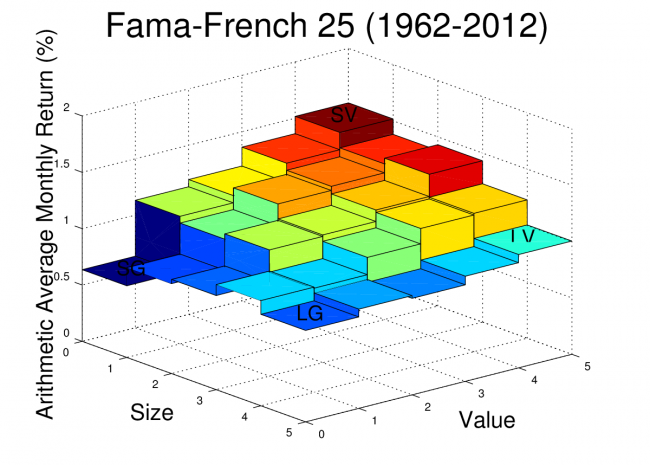
For reference, the arithmetic average monthly returns of the FF25 portfolios are plotted for the date range used in this analysis. The Octave script to create this plot was provided in an earlier post.
Principal Component Analysis Example
PCA is a method for constructing factors which are uncorrelated with each other and which allow us to maximize R^2 when running regressions on the target portfolios. We can find the PCA factors with just a few lines of Octave code!
Step 1: Construct a matrix of excess returns
If we have a set of portfolios, we can show the returns in a matrix where each column is a portfolio and each row is a return.
For example, if I have 25 portfolios with 612 months of return data, I can structure these returns in a 612 by 25 matrix, where the first row is the earliest return for each portfolio. Generally, when working with equity return factor models, the monthly risk-free rate is deducted from each monthly return, so the returns used are excess returns.
For this example, I have “preassembled” the excess return matrix and I read it in from a text file with the following Octave command:
rx = load(‘excessreturns.txt’)
Step 2: Calculate the Covariance Matrix
The Octave function “cov” can be used to calculate the covariance matrix for our return data.
Sigma_rx=cov(rx)
Step 3: Calculate the Eigenvalue Decomposition
Once we have the covariance matrix, we can use Octave to find the eigenvalue decomposition using the “eig” function:
[V,Lambda]=eig(Sigma)
The V columns are the eigenvectors and the diagonal elements of Lambda are the eigenvalues.
Step 4: Sort by Largest Standard Deviation and Extract Factor Loads
We need to sort the eigenvalues so that we can determine which factors will capture the highest variance of the data, so we first pull out the diagonal elements of Lambda and sort from largest to smallest. This sort order is then applied to the eigenvectors.
[stdevs,order]=sort(diag(Lambda)’.^0.5,’descend’)
V = V(:,order)
Note that I’m taking the square root, so the variances become standard deviations. This step is not necessary, but I like to look at the standard deviations rather than the variances when plotting. The standard deviations for each vector can be plotted using the “bar” command.
bar(stdevs)
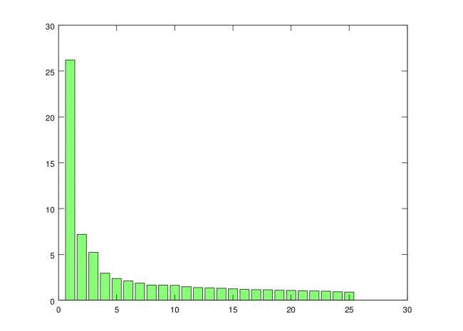
You can see that standard deviation captured by each additional factor trails off rapidly. So, for this analysis, I’m just going to use the first three factors.
Step 5: Calculate the PCA Factors
The columns of V are the eigenvectors, and we sorted V so the eigenvectors accounting for the greatest variance in the data are ordered first. Since the eigenvector column can be interpreted as a factor load for each of our original portfolios, we can create the factors themselves with a matrix multiplication. Note that I don’t “center” the matrix rx, which is usually done for PCA. In this case, I want to retain the mean because these new factors are essentially portfolio returns, and I want to be able to get meaningful alphas when I use them in regressions.
factors = rx*V
The first three factors that we are interested in will be the first three columns of the new factors matrix.
f1 = factors(:,1)
f2 = factors(:,2)
f3 = factors(:,3)
We now have our three PCA factors!
Example Code (Simple Version):
rx = load('excessreturns.txt');                        % Load Excess Returns
Sigma_rx = cov(rx);                                    % Calculate covariance matrix of excess returns</em>
[V,Lambda]=eig(Sigma_rx);                              % Eigenvalue decomposition
[stdevs,order] = sort(diag(Lambda)'.^0.5,'descend');   % Sort standard deviations in decending order
bar(stdevs)                                            % Plot standard deviations to see importance of each factor
V = V(:,order);                                        % Sort Eigenvectors in similar way
factors = rx*V;                                        % Calculate Factors
f1 = factors(:,1);                                     % Extract Factor 1
f2 = factors(:,2);                                     % Extract Factor 2
f3 = factors(:,3);                                     % Extract Factor 3
The First Three PCA Factors and Factor Loads for the FF25
The first three PCA factors generated by the script above can be used to analyze portfolios in a manner similar to the Fama-French factors. However, unlike the Fama-French factors, the PCA factors do not have a simple interpretation such as “size” or “value”. Nevertheless, Arbitrage Pricing Theory suggests that we should see small alphas if the R^2 for the regression is high.
For reference, I’ve posted the three PCA equity factors in a Google Docs Spreadsheet. It is an interesting exercise to run some regressions using these factors and to compare the results with the FF3F model. The PCA factors should be expected to give higher R^2 for the FF25 portfolios since they are optimized to fit that data, but the results could be better or worse when tested on other types of portfolios.
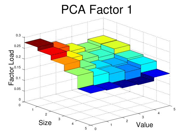
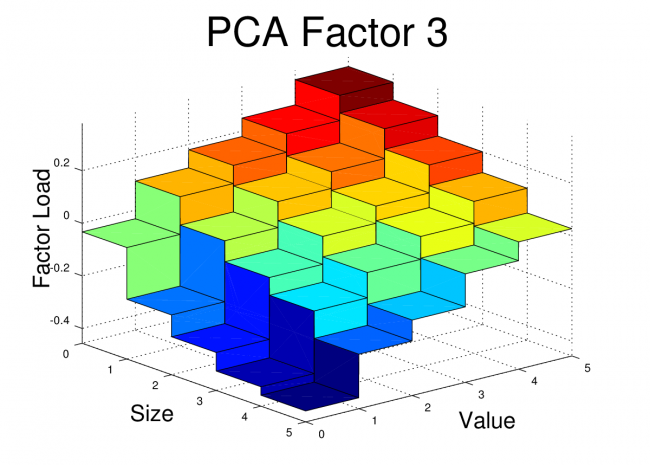
For the FF25 portfolios, we don’t need to run any regressions to get the factor loads. The factor loads for each PCA factor are simply the corresponding columns of V.
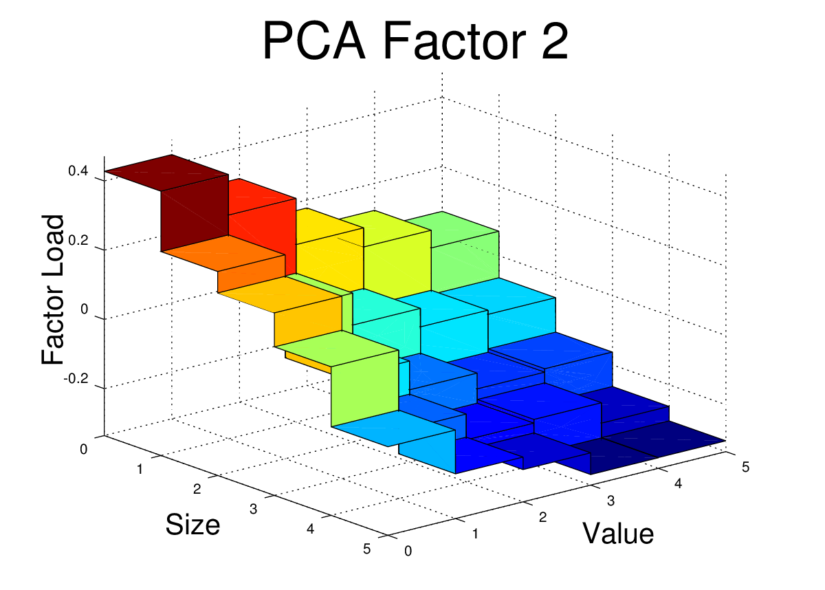
I’ve plotted the FF25 factor loads for the first three PCA equity factors here. The code to generate these plots is shown at the end of this post.
 Conclusion

At first glance, these PCA factor loads for the FF25 don’t bear much resemblance to what we would see with the FF3F model. For example, we would expect HML to have a loading which was relatively flat along the size axis, but which increased as we moved towards higher “value”. We would expect SMB loadings to be relatively flat across the value dimension, but to step up as we moved towards smaller size.
However, the PCA factors have certain properties that real world risk factors won’t necessarily have. The PCA factors are uncorrelated, they are normalized, and each in turn captures as much of the remaining covariance as possible. So, even if the PCA is successfully picking up covariance caused by real risk there may be equally effective factors (effective in terms of getting low alpha and high R^2) which are linear combinations of these PCA factors. In fact, some linear combination of these three factors may give use something very similar to the FF3F factors. In the next post, I’ll dig into this idea further.
Example Code (Extended Version):
Main Script:
clear all;
close all;

% Load Factors and Portfolio Returns
% The target files are the files from the Kenneth French website with comment text and data other than monthly returns

removed.
ff_facts = load('F-F_Research_Data_Factors_monthly.txt');
ff_ports = load('25_Portfolios_5x5_monthly.txt');

% Determine Start and Stop points for FF factors
% 1962 chosen so that only Compustat era data is used
start_year = 1962;
start_month = 1;
stop_year = 2012;
stop_month = 12;
start = (start_year-1932)*12 + (start_month-1) + 67;
stop = (stop_year-1932)*12 + (stop_month-1) + 67;

% Pullout risk free rate starting on start date
rf = ff_facts(start:stop,5);

% Pull out FF25 Portfolio Returns for Specified Date Range
x = ff_ports(start:stop,:); % start after NAs end i.e line 67
r = x(:,2:end);             % remove first column which is dates
rx = r - repmat(rf,1,25);   % calculate excess returns for portfolios

Sigma_rx = cov(rx);                                   % Calculate covariance matrix of excess returns
[V,Lambda]=eig(Sigma_rx);                             % Eigenvalue decomposition
[stdevs,order] = sort(diag(Lambda)'.^0.5,'descend');  % Sort standard deviations in decending order
bar(stdevs)                                           % Plot standard deviations to see importance of each factor
print -dpng scree.png                                 % Print to file
V = V(:,order);                                       % Sort Eigenvectors in similar way
factors = rx*V;                                       % Calculate Factors
f1 = factors(:,1);                                    % Extract Factor 1
f2 = factors(:,2);                                    % Extract Factor 2
f3 = factors(:,3);                                    % Extract Factor 3

% Create 3-D Plots of Factor Loadings (Columns of V)

figure;
fivebyfive(V(:,1));
xlabel('Size','fontsize',20)
ylabel('Value','fontsize',20)
zlabel('Factor Load','rotation',90,'fontsize',20)
title('PCA Factor 1','fontsize',36)
view(50,25)
print -dpng pca1.png

figure;
fivebyfive(V(:,2));
xlabel('Size','fontsize',20)
ylabel('Value','fontsize',20)
zlabel('Factor Load','rotation',90,'fontsize',20)
title('PCA Factor 2','fontsize',36)
view(50,25)
print -dpng pca2.png

figure;
fivebyfive(V(:,3));
xlabel('Size','fontsize',20)
ylabel('Value','fontsize',20)
zlabel('Factor Load','rotation',90,'fontsize',20)
title('PCA Factor 3','fontsize',36)
view(50,25)
print -dpng pca3.png

% Write Factors to file
dates = x(:,1);
pcafactors = [dates f1 f2 f3 rf];
save -ascii pcafactors.txt pcafactors
Function used by main script. This script should be saved in the working directory as “fivebyfive.m”.
function[] = fivebyfive(zvalues);

% Expand 5x5 data to 10x10 for use in surface plot function
zvals = [zvalues' ; zvalues'];
zvals = reshape(zvals,10,5);
zvals = [zvals;zvals];
zvals = reshape(zvals,10,10);

% Define x and y values
x = [0 0.999 1 1.999 2 2.999 3 3.999 4 5];
y = [0 0.999 1 1.999 2 2.999 3 3.999 4 5];

% Create x-y mesh for surface plot
[xx,yy] = meshgrid(x,y);

% Generate Plot
surf(xx,yy,zvals)
xlabel('Size','fontsize',20)
ylabel('Value','fontsize',20)
zlabel('Factor Load','rotation',90,'fontsize',20)
axis([0 5 0 5 min(0,min(zvalues)-0.1*abs(min(zvalues))) max(zvalues)+0.1*abs(max(zvalues))])
I am trying to understand PCA and found this very helpful. My question is: of the 25 portfolios used, which 3 were used as the final factors?
It is the first three factors that he used for 3D plots but the linear combination of them (selecting optimal weights for the three factors) to obtain similar 3D plot to FF3F.
My understanding is that all 25 portfolios were used for factor calculation