Warning: "continue" targeting switch is equivalent to "break". Did you mean to use "continue 2"? in /home/calcul9/public_html/wp-content/themes/suffusion/functions/media.php on line 580

Warning: "continue" targeting switch is equivalent to "break". Did you mean to use "continue 2"? in /home/calcul9/public_html/wp-content/themes/suffusion/functions/media.php on line 583

Warning: "continue" targeting switch is equivalent to "break". Did you mean to use "continue 2"? in /home/calcul9/public_html/wp-content/themes/suffusion/functions/media.php on line 586

Warning: "continue" targeting switch is equivalent to "break". Did you mean to use "continue 2"? in /home/calcul9/public_html/wp-content/themes/suffusion/functions/media.php on line 589

Warning: "continue" targeting switch is equivalent to "break". Did you mean to use "continue 2"? in /home/calcul9/public_html/wp-content/themes/suffusion/functions/media.php on line 592
2013 March » The Calculating Investor

About two years ago, I posted some region by region plots of the Case-Shiller home price data. I thought it would be interesting to re-run those plots to see how things have changed since 2011.

The plots below show the housing price history for major cities within each region. Each plot also includes the 20 city average data series.  Each city’s price history is normalized to 100 in January 2000.  Since the Case-Shiller data is not adjusted for inflation, I also added a normalized CPI-U series to each plot.

The “Mortgage Payment” plot shows the price indices adjusted to account for changing mortgage rates.  This plot incorporates both the Case-Shiller data and the mortgage rate to show how the payments for a 30 year fixed rate mortgage have varied for a “constant-quality” home.

northeast_shiller Continue reading »

In my previous post, I showed how to create equity return factors using principal component analysis. In this post, I’m going to compare the three PCA factors I created to the three Fama-French factors.

The goal of this post is to determine whether or not the Fama-French factors are leaving anything significant on the table that the PCA factors, which capture as much covariance in the target portfolios as is possible with three factors, are able to pick up.

In other words, I’ll be comparing the R^2s and alphas for both the Fama-French factors and the PCA factors, and, after some re-arranging, I’ll also compare the factor loadings.

Data

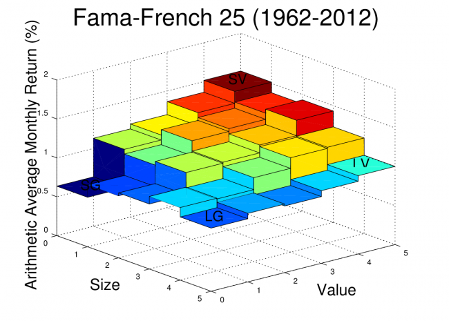
The Fama-French 3 Factor (FF3F) data and the Fama-French 25 size and value sorted portfolio (FF25) data come from the Kenneth French website.  The PCA factors were calculated in the previous post, and I posted the data in a Google Docs Spreadsheet.

R^2 and Alpha using PCA Factors and Fama French Factors

As a first step, the R^2s and alphas for the FF25 portfolios can be calculated using both the Fama-French factors and the PCA factors.

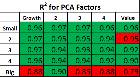
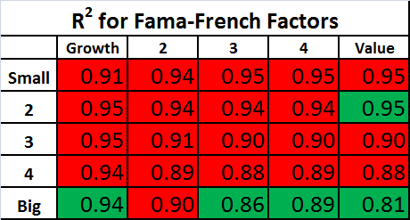
The PCA factors will give us the best fit across the 25 portfolios that is possible with three factors, so we expect the R^2s for the Fama-French factors to be lower on average. The question is: How much lower?

The tables below show the R^2s for the PCA Factors and Fama-French Factors.  For each table, the values highlighted in green have an R^2 which is higher than the alternative model, and the values highlighted in red have an R^2 which is lower than the alternative model.

pcarsquared

ffrsquared Continue reading »

The most popular “factors” for analyzing equity returns are the three Fama-French factors (RMRF, HML and SMB).  The RMRF factor is the market return minus the risk free rate, and the HML and SMB factors are created by sorting portfolios into several “value” and “size” buckets and forming long-short portfolios.

The three factors can be used to explain, though not predict, the returns for a variety of diversified portfolios. Many posts on this blog use the Fama-French 3 Factor (FF3F) model, including a tutorial on running the 3-factor regression using R.

An alternative way to construct factors is to use linear algebra to create “optimal” factors using a technique such as principal component analysis (PCA). This post will show how to construct the statistically optimal factors for the Fama-French 25 portfolios (sorted by size and value).

In my next post, I will compare these PCA factors to the Fama-French factors.

Description of Data

The data used for this analysis comes from the Kenneth French website.  I’m using the Fama-French 25 (FF25) portfolio returns which are available in the file titled “25 Portfolios Formed on Size and Book-to-Market”.  I’m using the returns from 1962 through 2012 since the pre-Compustat era portfolios have relatively few stocks.

The Fama-French factors are also available on the Kenneth French website in the file titled “Fama/French Factors”.  In this post, I will use not use the Fama-French factors themselves, but I do use the factor data file to get the monthly risk-free rate.

For reference, the arithmetic average monthly returns of the FF25 portfolios are plotted for the date range used in this analysis.  The Octave script to create this plot was provided in an earlier post.

port24avgs

Continue reading »